Classification

Scikit-Learn offers various utilities for accessing and generating datasets. The MNIST dataset can be fetched from OpenML using fetch_openml. For example,

from sklearn.datasets import import fetch_openml
mnist = fetch_openml('mnist_784', as_frame=False)

• fetch_openml()
  → Downloads real-world datasets from OpenML.org. Returns input features and labels.
  → By default, returns data in pandas.DataFrame format. Use as_frame=False to get NumPy arrays instead.

• load_* functions
  → Load small built-in toy datasets (no internet download required).

• make_* functions
  → Generate synthetic datasets for testing and debugging purposes.

• Returns are usually in (X, y) format as NumPy arrays. Some datasets come as sklearn.utils.Bunch objects — dictionary-like with dot-access.

Common Bunch Keys

• "DESCR" – Description of the dataset
• "data" – Feature matrix (usually 2D NumPy array)
• "target" – Labels (usually 1D NumPy array)

Notes

• Datasets returned by fetch_openml() are not always shuffled or split.
• Shuffling may be a bad idea in some contexts—for example, if you are working on time series data (such as stock market prices or weather conditions)

Training a Binary Classifier

We simplify the MNIST task to a binary classification problem: identifying whether a digit is a 5 or not (True/False). The SGDClassifier is well-suited for this as it uses stochastic gradient descent (SGD), allowing it to scale efficiently to large datasets and process instances one at a time—ideal for online learning.

y_train_5 = (y_train == '5')  # True for all 5s, False otherwise
y_test_5 = (y_test == '5')
from sklearn.linear_model import SGDClassifier

sgd_clf = SGDClassifier(random_state=42)
sgd_clf.fit(X_train, y_train_5)

Evaluating Classifier Accuracy with Cross-Validation Classifier evaluation can be trickier than regression. A common method is k-fold cross-validation using cross_val_score(). Below is a 3-fold example using accuracy as the metric.

from sklearn.model_selection import cross_val_score
cross_val_score(sgd_clf, X_train, y_train_5, cv=3, scoring="accuracy")
# Output: array([0.95035, 0.96035, 0.9604])

However, high accuracy can be misleading if the dataset is imbalanced.

A DummyClassifier that always predicts "not 5" can still achieve over 90% accuracy, highlighting why accuracy alone is not enough.

from sklearn.dummy import DummyClassifier

dummy_clf = DummyClassifier()
dummy_clf.fit(X_train, y_train_5)
print(any(dummy_clf.predict(X_train)))  # prints False

We use the DummyClassifier to detect misleading high accuracy. In the example,

• The model gets 95% accuracy predicting whether a digit is 5.
• But only 5% of images are 5 — so predicting “not 5” every time already gives 95% accuracy.
• DummyClassifier helps you reveal this trick — it matches the high score without any learning.

A much better way to evaluate the performance of a classifier is to look at the confusion matrix (CM).

Confusion Matrices for Classifier Evaluation

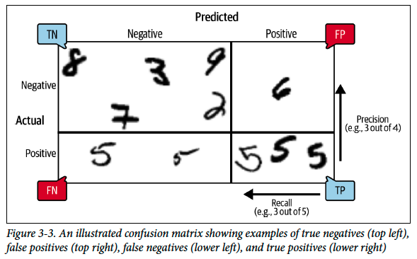
A confusion matrix summarizes how well a classifier is performing by counting correct and incorrect predictions for each class. Each row represents an actual class, and each column a predicted class.

Instead of evaluating on the test set (which should be reserved for final evaluation), we use cross_val_predict() to generate predictions via cross-validation without ever training on the data it’s predicting.

from sklearn.model_selection import cross_val_predict

y_train_pred = cross_val_predict(sgd_clf, X_train, y_train_5, cv=3)

This returns predictions for each training instance as if they were 'unseen' by the model.

from sklearn.metrics import confusion_matrix

cm = confusion_matrix(y_train_5, y_train_pred)
cm
# Output:
# array([[53892,   687],
#        [ 1891,  3530]])

Precision: A Metric from the Confusion Matrix

While a confusion matrix gives a detailed picture of classification results, precision offers a more concise metric — it measures the accuracy of positive predictions only. Precision is defined as the ratio of true positives to all predicted positives:

$$\text{precision} = \frac{TP}{TP + FP}$$

Where:

• TP: True Positives — correctly predicted positive instances
• FP: False Positives — instances wrongly predicted as positive

A naive way to get perfect precision is to predict positive only once — and only when you're sure it’s correct. This avoids false positives entirely but isn’t practical as it sacrifices recall (you’ll miss most positives).

We also consider recall, which measures how many actual positives were correctly predicted.

$$\text{recall} = \frac{TP}{TP+FN}$$

• TP: True Positives — correctly predicted positive instances
• FN: False Negatives — actual positives the classifier missed High recall means fewer positive cases go undetected, which is important in tasks like medical diagnostics or fraud detection.

Scikit-Learn provides functions to compute classifier metrics like precision, recall, and the F₁ score. Precision measures the accuracy of positive predictions, and recall measures the ability to find all positive instances. The F₁ score combines both into a single metric — the harmonic mean — and favors classifiers that balance both precision and recall.

from sklearn.metrics import precision_score, recall_score

precision_score(y_train_5, y_train_pred)
# == 3530 / (687 + 3530) ≈ 0.837089772350012
recall_score(y_train_5, y_train_pred)
# == 3530 / (1891 + 3530) ≈ 0.6511713705958311

F₁ Score

The F₁ score is computed as:

$$F_1 = 2 \times \frac{\text{precision} \times \text{recall}}{\text{precision}+\text{recall}} = \frac{TP}{TP+\frac{FN+FP}{2}}$$

It is useful when you need a single score to compare classifiers, especially when you care equally about precision and recall.

from sklearn.metrics import f1_score

f1_score(y_train_5, y_train_pred)
# ≈ 0.7325171197343846

Precision/Recall Trade-Off

• F₁ score favors balance between precision and recall.
• However, in some applications, one may be more important than the other:
  • E.g., For filtering kids' videos → prioritize precision
  • E.g., For catching shoplifters → prioritize recall
• You can’t maximize both at the same time — improving one usually worsens the other. This is called the precision/recall trade-off.

The SGDClassifier computes a decision score for each instance using its decision_function(). This score is compared to a threshold to determine the predicted class. If the score is above the threshold, the instance is labeled positive; otherwise, it's negative.

Adjusting this decision threshold allows you to shift the balance between precision and recall:

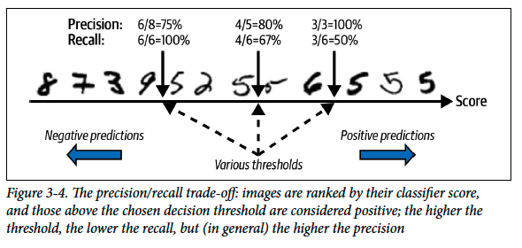
• Raising the threshold: increases precision, decreases recall
• Lowering the threshold: increases recall, decreases precision

This trade-off is crucial in applications where one metric is more important than the other.

# Access decision scores instead of predictions
y_scores = sgd_clf.decision_function([some_digit])
y_scores
# array([2164.22030239])

# Default threshold (same as using predict)
threshold = 0
y_some_digit_pred = (y_scores > threshold)
# array([ True ])

# Raise the threshold to make the classifier stricter
threshold = 3000
y_some_digit_pred = (y_scores > threshold)
# array([ False ])

Choosing the Right Threshold Using Precision/Recall Curve

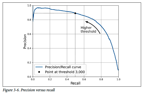
To tune the decision threshold, use cross_val_predict() with method="decision_function" to retrieve decision scores. Then use precision_recall_curve() to get precision and recall values at various thresholds. You can visualize the trade-off using a plot.

# Get decision scores using cross-validation
y_scores = cross_val_predict(sgd_clf, X_train, y_train_5, cv=3,
                             method="decision_function")

# Compute precision and recall at all thresholds
from sklearn.metrics import precision_recall_curve
precisions, recalls, thresholds = precision_recall_curve(y_train_5, y_scores)

# Plot precision and recall vs. thresholds
plt.plot(thresholds, precisions[:-1], "b--", label="Precision", linewidth=2)
plt.plot(thresholds, recalls[:-1], "g-", label="Recall", linewidth=2)
plt.vlines(threshold, 0, 1.0, "k", "dotted", label="threshold")
# Beautify the figure: add grid, legend, axis, labels, and circles
plt.show()

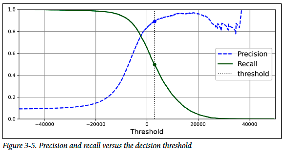
• The precision curve is bumpy because precision may drop when adding a false positive.
• The recall curve is smooth because recall only decreases as the threshold increases.
• This plot helps you choose a threshold that balances both metrics depending on your task.

Another way to select a good precision/recall trade-off is to plot precision directly against recall.

ROC Curve

The Receiver Operating Characteristic (ROC) curve is a tool to evaluate binary classifiers by plotting the True Positive Rate (TPR, or recall) against the False Positive Rate (FPR, or fall-out). The FPR is calculated as 1 - specificity, where specificity is the True Negative Rate (TNR). The curve helps visualize the trade-off between TPR and FPR across various thresholds.

To plot the ROC curve, use the roc_curve() function to compute the TPR and FPR for different thresholds, and plot TPR vs. FPR using Matplotlib. The closer the curve is to the top-left corner, the better the classifier. A random classifier would lie along the diagonal line (from (0,0) to (1,1)). The area under the curve (AUC) can be used to summarize performance into a single number between 0.5 (random) and 1.0 (perfect).

from sklearn.metrics import roc_curve

fpr, tpr, thresholds = roc_curve(y_train_5, y_scores)

To identify the TPR and FPR at a specific threshold (e.g., the one corresponding to 90% precision):

idx_for_threshold_at_90 = (thresholds <= threshold_for_90_precision).argmax()
tpr_90 = tpr[idx_for_threshold_at_90]
fpr_90 = fpr[idx_for_threshold_at_90]

To calculate the AUC (Area Under Curve) of the ROC:

from sklearn.metrics import roc_auc_score

roc_auc_score(y_train_5, y_scores)
# Output: 0.96040938554008616

AUC offers a single metric to compare classifiers: the higher the AUC, the better. A good classifier should have an ROC curve that stays far from the diagonal line (random performance) and close to the top-left corner.

Choosing Between ROC and PR Curves

Since the ROC and precision/recall (PR) curves are closely related, a common question is: when should you use one over the other?

• Use the PR curve when:
  • The positive class is rare, or
  • You care more about false positives than false negatives
• Use the ROC curve in other cases, especially when:
  • The classes are more balanced
  • You care equally about TPR and FPR

In imbalanced datasets (e.g., few 5s vs. many non-5s), the ROC curve may appear overly optimistic. The PR curve better reveals whether the model could still be improved — e.g., if it could be closer to the top-right corner, indicating higher precision and recall.

Comparing PR Curves with RandomForestClassifier

To compare the PR curve and F₁ score of RandomForestClassifier with those of SGDClassifier, we must first train the random forest model and compute a score for each instance.

Unlike SGDClassifier, RandomForestClassifier does not have a decision_function(), but it does offer predict_proba() which returns class probabilities. You can use the probability of the positive class as the decision score. This works well for functions like precision_recall_curve().

To obtain probability predictions via cross-validation, use cross_val_predict() with method="predict_proba":

from sklearn.ensemble import RandomForestClassifier

forest_clf = RandomForestClassifier(random_state=42)

y_probas_forest = cross_val_predict(forest_clf, X_train, y_train_5, cv=3, method="predict_proba")

To inspect class probabilities for the first two training samples:

y_probas_forest[:2]
array([[0.11, 0.89], [0.99, 0.01]])

These results indicate the model predicts the first image is a 5 with 89% probability and the second is not a 5 with 99% probability. Since the outputs are probabilities for each class, each row sums to 1.

Plotting and Comparing PR Curves for Random Forest and SGD Classifiers

The predicted values from predict_proba() are estimated probabilities, not actual probabilities. These estimates can be miscalibrated—either too high or too low. The sklearn.calibration package provides tools to better align predicted probabilities with real-world outcomes.

To compute and plot the precision-recall (PR) curve for the random forest classifier, we extract the second column (positive class probabilities) and use the precision_recall_curve() function:

y_scores_forest = y_probas_forest[:, 1]

precisions_forest, recalls_forest, thresholds_forest = precision_recall_curve(
    y_train_5, y_scores_forest)

Multiclass Classification

Multiclass classifiers (a.k.a. multinomial classifiers) can distinguish between more than two classes, unlike binary classifiers. Some classifiers like LogisticRegression, RandomForestClassifier, and GaussianNB support multiclass classification natively. Others (e.g., SGDClassifier, SVC) are strictly binary, but you can use strategies like:

• One-vs-Rest (OvR): Train one binary classifier per class (e.g., 10 classifiers for digits 0–9). Each outputs a score, and the highest-scoring class is selected.
• One-vs-One (OvO): Train one classifier per pair of classes. If there are ( N ) classes, you need ( N \times (N-1)/2 ) classifiers. For MNIST (10 classes), this means 45 classifiers. Each class is compared in a "duel", and the class that wins the most is chosen.

OvO is preferred for small training sets, while OvR works better with large sets and is preferred by most binary classification algorithms.

from sklearn.svm import SVC

svm_clf = SVC(random_state=42)
svm_clf.fit(X_train[:2000], y_train[:2000]) # y_train, not y_train_5

Multiclass Classification: OvO, OvR, and Class Label Lookups

When a classifier is trained, it stores the list of target class labels in the classes_ attribute. For MNIST, the index usually matches the label itself, but this is not guaranteed. You can access the class label using:

svm_clf.classes_
array(['0', '1', '2', '3', '4', '5', '6', '7', '8', '9'], dtype=object)

svm_clf.classes_[class_id]
'5'

To explicitly choose a strategy, Scikit-Learn provides OneVsOneClassifier and OneVsRestClassifier. The code below wraps an SVC in a OneVsRestClassifier:

from sklearn.multiclass import OneVsRestClassifier

ovr_clf = OneVsRestClassifier(SVC(random_state=42))
ovr_clf.fit(X_train[:2000], y_train[:2000])

Using SGDClassifier on Multiclass Data

Training an SGDClassifier on a multiclass dataset uses the One-vs-Rest (OvR) strategy by default:

sgd_clf = SGDClassifier(random_state=42)
sgd_clf.fit(X_train, y_train)

The classifier assigns one score per class using decision_function():

sgd_clf.decision_function([some_digit]).round()
array(-31893., -34420.,  -9531.,  1824., -22320.,  -1386., -26189.,
        -16148., -4064., -12051.)

The model predicts the class with the highest score. Use cross_val_score() to evaluate accuracy:

cross_val_score(sgd_clf, X_train, y_train, cv=3, scoring="accuracy")
array([0.87365, 0.85835, 0.8689])

Accuracy is over 85%. Scaling the data improves performance:

from sklearn.preprocessing import StandardScaler

scaler = StandardScaler()
X_train_scaled = scaler.fit_transform(X_train.astype("float64"))

>>> cross_val_score(sgd_clf, X_train_scaled, y_train, cv=3, scoring="accuracy")
array([0.8983, 0.891 , 0.9018])

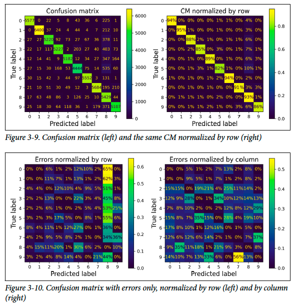
After identifying a promising model, error analysis helps you improve it further by inspecting misclassifications. This is commonly done using a confusion matrix.

To plot a colored and more interpretable confusion matrix, use ConfusionMatrixDisplay.from_predictions():

from sklearn.metrics import ConfusionMatrixDisplay

y_train_pred = cross_val_predict(sgd_clf, X_train_scaled, y_train, cv=3)
ConfusionMatrixDisplay.from_predictions(y_train, y_train_pred)
plt.show()```

This shows where the model confuses digits, like mistaking 5s for 8s. To improve readability, normalize by row using `normalize="true"` and optionally format percentages with `values_format=".0%"`:

```python
ConfusionMatrixDisplay.from_predictions(y_train, y_train_pred,
                                        normalize="true", values_format=".0%")
plt.show()

To visualize only the errors, assign a sample weight of 0 to correct predictions:

sample_weight = (y_train_pred != y_train)
ConfusionMatrixDisplay.from_predictions(y_train, y_train_pred,
                                        sample_weight=sample_weight,
                                        normalize="true", values_format=".0%")
plt.show()

This highlights which digits are most often confused. For instance, many 8s are confused with 9s, and 56% of misclassified 7s are actually 9s. This information suggests where to focus your model improvement efforts—e.g., reducing false 8s by gathering more training data, adding shape-based features, or using preprocessing techniques (like Scikit-Image or Pillow) to highlight distinguishing patterns such as closed loops.

Multilabel Classification

In multilabel classification, each instance can belong to multiple classes simultaneously. For example, in face recognition, a model might tag an image with multiple names if it detects more than one known person. This is handled by assigning multiple binary labels per instance.

The example below constructs a simple multilabel classifier using KNeighborsClassifier, assigning two binary labels: whether a digit is large (≥7) and whether it is odd.

import numpy as np
from sklearn.neighbors import KNeighborsClassifier

y_train_large = (y_train >= 7)
y_train_odd = (y_train.astype("int8") % 2 == 1)
y_multilabel = np.c_[y_train_large, y_train_odd]

knn_clf = KNeighborsClassifier()
knn_clf.fit(X_train, y_multilabel)

knn_clf.predict([some_digit])
# Output: array(False,  True)

To evaluate multilabel classifiers, one option is to compute the average F₁ score across all labels, which treats each label equally:

y_train_knn_pred = cross_val_predict(knn_clf, X_train, y_train_multilabel, cv=3)
f1_score(y_multilabel, y_train_knn_pred, average="macro")
# Output: 0.976410265656065

If label importance varies, use average="weighted" in f1_score() to account for label support.

For classifiers that don’t natively support multilabel classification (e.g., SVC), an alternative is to train one binary classifier per label. However, label dependencies (e.g., large digits are more likely to be odd) may lead to suboptimal results. To fix this, ClassifierChain can be used. It chains multiple models together, feeding each model not only the input features but also the predictions of earlier models.

from sklearn.multioutput import ClassifierChain

chain_clf = ClassifierChain(SVC(), cv=3, random_state=42)
chain_clf.fit(X_train[:2000], y_multilabel[:2000])

chain_clf.predict([some_digit])
# Output: array(0., 1.)

Multioutput Classification

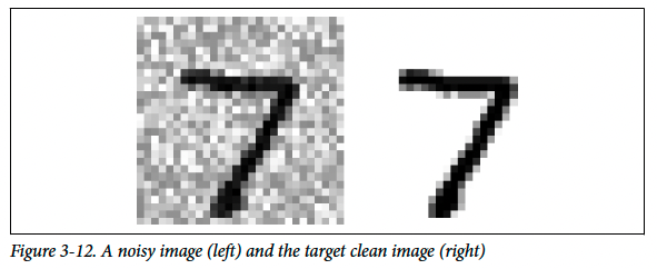
Multioutput–multiclass classification (or simply multioutput classification) is an extension of multilabel classification where each label can take multiple values instead of just binary ones. An example of this is a denoising system: given a noisy image as input, the classifier outputs a clean image, where each pixel is a separate label with intensity values (0–255), making it a multioutput classification task.

Although this task resembles regression, it's framed as classification here since pixel intensities take on discrete values. Multioutput systems can be used for both classification and regression purposes.

To implement this, we use the MNIST dataset, add random noise to the training and test sets using NumPy's randint(), and attempt to train a model that maps noisy digits to their clean counterparts.

np.random.seed(42)  # to make this code example reproducible
noise = np.random.randint(0, 100, (len(X_train), 784))
X_train_mod = X_train + noise
noise = np.random.randint(0, 100, (len(X_test), 784))
X_test_mod = X_test + noise

y_train_mod = X_train
y_test_mod = X_test

Then we train a KNeighborsClassifier on the noisy-clean image pairs and ask it to clean up a noisy image:

knn_clf = KNeighborsClassifier()
knn_clf.fit(X_train_mod, y_train_mod)
clean_digit = knn_clf.predict([X_test_mod[0]])
plot_digit(clean_digit)
plt.show()