Ensemble Learning and Random Forests

Ensemble Learning and Random Forests

A group of predictors is called an ensemble, the technique is called ensemble learning, and an algorithm using this approach is called an ensemble method.

A common example is training many decision tree classifiers on different random subsets of the training set. Each tree makes its own prediction, and the class with the most votes becomes the ensemble’s final prediction. This type of decision-tree ensemble is called a random forest, which is simple but considered one of the most powerful machine learning algorithms.

Voting Classifiers

A voting classifier is an ensemble method that combines the predictions of several different classifiers, such as logistic regression, SVM classifier, random forest, and k-nearest neighbors. Instead of relying on only one model, it aggregates the predictions of multiple models. When the final prediction is the class that receives the most votes, this is called a hard voting classifier.

A hard voting classifier can often achieve higher accuracy than the best individual classifier in the ensemble. This is possible even if each classifier is only a weak learner, meaning it performs only slightly better than random guessing. The ensemble can become a strong learner if there are enough weak learners and their errors are sufficiently independent.

Law of Large Numbers

Definition. Law of Large Numbers If $X_1, X_2, \dots, X_n$ are independent and identically distributed random variables with expected value $\mu = \mathbb{E}[X_i]$, then the sample mean $\bar{X}_n = \frac{1}{n}\sum_{i=1}^{n} X_i$ converges to the expected value $\mu$ as $n$ becomes large: $\bar{X}_n \to \mu$. More formally, for any $\varepsilon > 0$,

$$P(|\bar{X}_n - \mu| > \varepsilon) \to 0 \quad \text{as } n \to \infty$$

Note. >Ensemble methods work best when the predictors are as independent from one another as possible. One way to create more diverse classifiers is to train them using very different algorithms. This increases the chance that each model will make different types of errors, which improves the ensemble’s overall accuracy.

from sklearn.datasets import make_moons
from sklearn.ensemble import RandomForestClassifier, VotingClassifier
from sklearn.linear_model import LogisticRegression
from sklearn.model_selection import train_test_split
from sklearn.svm import SVC

X, y = make_moons(n_samples=500, noise=0.30, random_state=42)
X_train, X_test, y_train, y_test = train_test_split(X, y, random_state=42)

voting_clf = VotingClassifier(
    estimators=[
        ('lr', LogisticRegression(random_state=42)),
        ('rf', RandomForestClassifier(random_state=42)),
        ('svc', SVC(random_state=42))
    ]
)
voting_clf.fit(X_train, y_train)

• voting_clf.fit(X_train, y_train) - fits the VotingClassifier by cloning every estimator and training the cloned models.
• voting_clf.estimators - returns the original estimators passed to the VotingClassifier.
• voting_clf.estimators_ - returns the fitted cloned estimators after training.
• voting_clf.named_estimators - returns the original estimators as a dictionary using their assigned names.
• voting_clf.named_estimators_ - returns the fitted cloned estimators as a dictionary using their assigned names.

Soft Voting

Soft voting uses the predicted class probabilities from each classifier. Instead of asking “which class did each model choose?”, it asks “how confident is each model for each class?”

For each class, Scikit-Learn averages the predicted probabilities across all classifiers, then chooses the class with the highest average probability. Mathematically, for a class $c$, the average probability for that class is $c=\frac{1}{m}\sum_{j=1}^{m}P_j(c\mid x)$. The ensemble predicts

$$\hat{y} = \arg\max_c \frac{1}{m} \sum_{j=1}^{m} P_j(c \mid x)$$

Bagging and Pasting

One way to create a diverse ensemble is to use the same training algorithm for every predictor, but train each predictor on a different random subset of the training set. This means the models have the same structure, such as all being decision tree classifiers, but each model sees a slightly different version of the data. Because each predictor learns from different samples, they may make different errors, which improves the ensemble when their predictions are aggregated.

Definition. Bagging Bagging, short for bootstrap aggregating, is an ensemble method where each predictor is trained on a random subset of the training set sampled with replacement.

Formally, given a training set $D = \{(x_i, y_i)\}_{i=1}^{n}$, bagging creates $B$ bootstrap datasets $D_1, D_2, \dots, D_B$, where each $D_b$ is sampled from $D$ with replacement. A predictor $h_b$ is trained on each $D_b$, and the final prediction is obtained by aggregating the predictions

$$\hat{y} = \text{mode}(h_1(x), h_2(x), \dots, h_B(x))$$

for classification, or

$$\hat{y} = \frac{1}{B}\sum_{b=1}^{B} h_b(x)$$

for regression.

Definition. Pasting Pasting is an ensemble method where each predictor is trained on a random subset of the training set sampled without replacement.

Formally, given a training set $D = \{(x_i, y_i)\}_{i=1}^{n}$, pasting creates $B$ random subsets $D_1, D_2, \dots, D_B$, where each $D_b$ is sampled from $D$ without replacement. Each predictor $h_b$ is trained on one subset, and the final prediction is obtained by majority voting for classification or averaging for regression.

In short, bagging allows the same training instance to appear multiple times in one subset, while pasting does not. Bagging and pasting can scale very well.

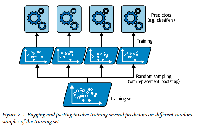
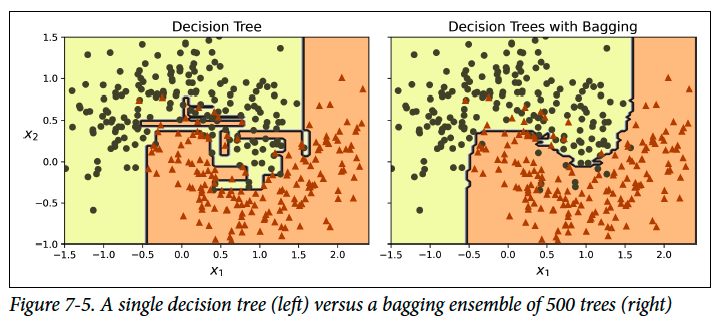
Each individual predictor may be weaker because it is trained on only part of the data, so it may have higher bias. But when many such predictors are combined, their different errors tend to cancel out, reducing variance and sometimes reducing bias as well. In practice, the ensemble often ends up with roughly similar bias but much lower variance than a single predictor trained on the full dataset.

Note. >A BaggingClassifier automatically performs soft voting instead of hard voting if the base classifier can estimate class probabilities using predict_proba(). This is true for decision tree classifiers, since they support probability estimates.

Bagging introduces a bit more diversity in the subsets that each predictor is trained on, so bagging ends up with a slightly higher bias than pasting; but the extra diversity also means that the predictors end up being less correlated, so the ensemble’s variance is reduced.

Out-of-Bag Evaluation

The training instances that are not sampled for a given predictor are called out-of-bag instances or OOB instances. Since these instances were not used to train that predictor, they can be used to evaluate it without needing a separate validation set.

If there are enough estimators, each training instance will likely be an OOB instance for several predictors. These OOB predictors can be used to make a fair prediction for that instance, and the ensemble’s accuracy or other metric can be computed from these predictions.

It can be shown mathematically that only about 63% of the training instances are sampled on average for each predictor.

Proof. Suppose the training set has $m$ instances, and bagging samples $m$ instances with replacement.

For one fixed training instance, the probability that it is not selected in one draw is $1 - \frac{1}{m}$.

Since there are $m$ independent draws, the probability that this instance is never selected is $\left( 1-\frac{1}{m}\right)^m$.

As $m$ becomes large:

$$\left(1 - \frac{1}{m}\right)^m \to e^{-1} \approx 0.3679$$

So the probability that the instance is selected at least once is:

$$1 - \left(1 - \frac{1}{m}\right)^m$$

For large $m$:

$$1 - e^{-1} \approx 1 - 0.3679 = 0.6321$$

□

Therefore, about $63.2\%$ of the training instances are sampled on average, while about $36.8\%$ are left out as out-of-bag instances.

In short, each bagging predictor trains on about $63\%$ of the unique training instances, while the remaining $37\%$ can be used for out-of-bag evaluation.

bag_clf = BaggingClassifier(DecisionTreeClassifier(), n_estimators=500, oob_score=True, max_samples=100, n_jobs=-1, random_state=42)
bag_clf.fit(X_train, y_train)
bag_clf.oob_score_

• oob_decision_function__ - the decision function for each training instance

Random Patches and Random Subspaces

BaggingClassifier can sample both training instances and input features. Instance sampling is controlled by max_samples and bootstrap, while feature sampling is controlled by max_features and bootstrap_features.

Definition. Random Patches Method The random patches method trains each predictor on a random subset of both the training instances and the input features. In short:

$$\text{Random patches} = \text{random rows} + \text{random columns}$$

Definition. Random Subspaces Method The random subspaces method trains each predictor on all training instances but only a random subset of the input features.

This is done by setting bootstrap=False, max_samples=1.0, and sampling features using bootstrap_features=True and/or max_features < 1.0.

Sampling features is especially useful for high-dimensional data, such as images, because it can speed up training and increase predictor diversity. However, it may increase bias slightly while reducing variance.

Random Forests

A random forest is an ensemble of decision trees, usually trained with bagging or sometimes pasting. Scikit-Learn provides RandomForestClassifier, which is more convenient and optimized for decision trees. For regression tasks, Scikit-Learn provides RandomForestRegressor.

from sklearn.ensemble import RandomForestClassifier

rnd_clf = RandomForestClassifier(n_estimators=500, max_leaf_nodes=16,
                                 n_jobs=-1, random_state=42)
rnd_clf.fit(X_train, y_train)

y_pred_rf = rnd_clf.predict(X_test)

A RandomForestClassifier has most of the hyperparameters of a DecisionTreeClassifier, which control how each tree grows, plus the hyperparameters of a BaggingClassifier, which control the ensemble itself.

By default, random forests samples $\sqrt{n}$ features, where $n$ is the total number of input features. This increases tree diversity, usually resulting in higher bias but lower variance, which often improves the overall model.

The following BaggingClassifier is roughly equivalent to the previous RandomForestClassifier:

bag_clf = BaggingClassifier(
    DecisionTreeClassifier(max_features="sqrt", max_leaf_nodes=16),
    n_estimators=500, n_jobs=-1, random_state=42)

Extra-Trees means Extremely Randomized Trees. It is like a random forest, but it adds even more randomness when growing each tree.

In a regular random forest:

• each split considers a random subset of features
• but it still searches for the best threshold for those features

In Extra-Trees:

• each split also considers a random subset of features
• but instead of searching for the best threshold, it chooses random thresholds
• then it picks the best split among those random choices

Because Extra-Trees does not spend as much time searching for the best split thresholds, it is usually faster to train than a regular random forest. However, this extra randomness usually means having more bias but lower variance.

Feature Importance

Random forests make it easy to measure the relative importance of each feature. Scikit-Learn measures feature importance by checking how much the tree nodes using that feature reduce impurity on average across all trees in the forest.

The importance score is a weighted average, where each node’s weight depends on the number of training samples associated with that node. After training, Scikit-Learn scales all feature importance scores so that their sum is equal to $1$.

Feature importance scores can be accessed using:

rnd_clf.feature_importances_

Example using the Iris dataset:

from sklearn.datasets import load_iris
from sklearn.ensemble import RandomForestClassifier

iris = load_iris(as_frame=True)

rnd_clf = RandomForestClassifier(n_estimators=500, random_state=42)
rnd_clf.fit(iris.data, iris.target)

for score, name in zip(rnd_clf.feature_importances_, iris.data.columns):
    print(round(score, 2), name)

Random forests are useful for quickly identifying which features matter most. This is especially helpful for feature selection, since unimportant features can potentially be removed to simplify the model.

Note. >Every time a feature is used in a node, Scikit-Learn checks how much that split reduced impurity. Big impurity reduction means the feature helped a lot. Small impurity reduction means the feature helped only a little.

Boosting

Boosting is an ensemble method that combines several weak learners into a strong learner. Unlike bagging or pasting, boosting trains predictors sequentially, where each new predictor tries to correct the errors made by the previous predictor.

Definition. Boosting Boosting is an ensemble technique where predictors are trained one after another, with each new predictor focusing more on the instances that previous predictors handled poorly.

AdaBoost

AdaBoost, short for adaptive boosting, trains predictors sequentially by increasing the weights of misclassified training instances. The first predictor is trained normally, then the incorrectly classified instances receive higher weights, forcing the next predictor to pay more attention to them. This process continues, making later predictors focus more on the hard cases.

Once all predictors are trained, the ensemble makes predictions similarly to voting, but each predictor has a different weight depending on its overall accuracy on the weighted training set. More accurate predictors have more influence on the final prediction.

Note. >AdaBoost is similar to gradient descent in spirit: instead of tweaking one model’s parameters to reduce a cost function, it gradually adds predictors to the ensemble to improve performance.

Warning. >A drawback of boosting is that training cannot be easily parallelized. Each predictor must wait for the previous predictor to finish training and be evaluated, so boosting does not scale as well as bagging or pasting.

Definition. Weighted Error Rate The weighted error rate of the $j^{th}$ predictor is the total weight of the training instances that it misclassifies.

Given training instances $\{(x^{(i)}, y^{(i)})\}_{i=1}^{m}$ with instance weights $w^{(i)}$, and predictions $\hat{y}_j^{(i)}$ from the $j^{th}$ predictor, the weighted error rate is:

$$r_j = \sum_{\hat{y}_j^{(i)} \neq y^{(i)}} w^{(i)}$$

Equivalently, using an indicator function:

$$r_j = \sum_{i=1}^{m} w^{(i)} \mathbf{1}\left(\hat{y}_j^{(i)} \neq y^{(i)}\right)$$

where $\mathbf{1}(\hat{y}_j^{(i)} \neq y^{(i)}) = 1$ if the instance is misclassified, and $0$ otherwise.

In AdaBoost, the weights are usually normalized so that $\sum_{i=1}^{m} w^{(i)} = 1$. This means the weighted error rate can be interpreted as the proportion of total instance weight assigned to mistakes.

In AdaBoost, each training instance starts with the same weight:

$$w^{(i)} = \frac{1}{m}$$

After training a predictor, AdaBoost computes the predictor’s weight $\alpha_j$. A more accurate predictor gets a larger weight, while a weak or mostly wrong predictor gets a smaller or even negative weight.

$$\alpha_j = \eta \log \frac{1 - r_j}{r_j}$$

Here, $r_j$ is the weighted error rate of the $j^{th}$ predictor, and $\eta$ is the learning rate. If $r_j$ is small, then $\alpha_j$ is large, meaning the predictor has more influence in the final prediction.

After computing $\alpha_j$, AdaBoost updates the instance weights. Correctly classified instances keep the same weight, while misclassified instances get boosted:

$$w^{(i)} \leftarrow \begin{cases} w^{(i)} & \text{if } \hat{y}_j^{(i)} = y^{(i)} \\ w^{(i)} \exp(\alpha_j) & \text{if } \hat{y}_j^{(i)} \neq y^{(i)} \end{cases}$$

The updated weights are then normalized so that they sum to $1$. A new predictor is trained using these updated weights, so it pays more attention to the instances that previous predictors misclassified.

The process repeats until the desired number of predictors is reached or a perfect predictor is found.

For prediction, AdaBoost combines all predictors using a weighted vote. Predictors with larger $\alpha_j$ have more influence:

$$\hat{y}(x) = \arg\max_k \sum_{\hat{y}_j(x)=k}^{N} \alpha_j$$

In short, AdaBoost trains predictors sequentially, increases the importance of misclassified instances, and combines all predictors using weighted majority voting.

AdaBoostClassifier with Decision Stumps

An AdaBoostClassifier commonly uses decision stumps as its base estimators. A decision stump is a very shallow decision tree with max_depth=1, meaning it has only one decision node and two leaf nodes. It is a weak learner, but AdaBoost combines many of them sequentially to form a stronger classifier.

from sklearn.ensemble import AdaBoostClassifier

ada_clf = AdaBoostClassifier(
    DecisionTreeClassifier(max_depth=1), n_estimators=30,
    learning_rate=0.5, random_state=42)
ada_clf.fit(X_train, y_train)

Note. >If an AdaBoost ensemble is overfitting the training set, try reducing n_estimators or increasing the regularization of the base estimator.

Gradient Boosting

Gradient boosting is a boosting method that trains predictors sequentially, with each new predictor trying to correct the errors made by the previous one. Unlike AdaBoost, which updates instance weights, gradient boosting fits each new predictor to the previous predictor’s residual errors.

Definition. Residual Error A residual error is the difference between the true target value and the model’s prediction.

$$\text{residual} = y - \hat{y}$$

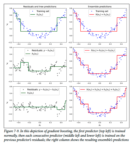
In gradient tree boosting, the base predictors are decision tree regressors. The first tree is trained on the original target values. The second tree is trained on the residual errors of the first tree. The third tree is trained on the residual errors left after combining the first two trees. The final prediction is made by adding the predictions of all trees.

import numpy as np
from sklearn.tree import DecisionTreeRegressor

np.random.seed(42)
X = np.random.rand(100, 1) - 0.5
y = 3 * X[:, 0] ** 2 + 0.05 * np.random.randn(100)  # y = 3x² + Gaussian noise

tree_reg1 = DecisionTreeRegressor(max_depth=2, random_state=42)
tree_reg1.fit(X, y)

y2 = y - tree_reg1.predict(X)
tree_reg2 = DecisionTreeRegressor(max_depth=2, random_state=43)
tree_reg2.fit(X, y2)

y3 = y2 - tree_reg2.predict(X)
tree_reg3 = DecisionTreeRegressor(max_depth=2, random_state=44)
tree_reg3.fit(X, y3)

After training, the ensemble predicts by summing the predictions of all trees:

X_new = np.array([[-0.4], [0.], [0.5]])
sum(tree.predict(X_new) for tree in (tree_reg1, tree_reg2, tree_reg3))

Scikit-Learn provides GradientBoostingRegressor for regression and GradientBoostingClassifier for classification. The following code creates the same kind of ensemble more directly:

from sklearn.ensemble import GradientBoostingRegressor

gbrt = GradientBoostingRegressor(max_depth=2, n_estimators=3,
                                 learning_rate=1.0, random_state=42)
gbrt.fit(X, y)

In short, gradient boosting builds an ensemble by repeatedly fitting new models to the remaining errors, so the ensemble’s predictions improve as more predictors are added.

Gradient Boosting Regularization

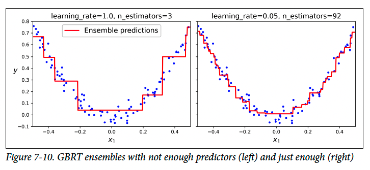
In Gradient Boosting, the learning_rate hyperparameter controls how much each tree contributes to the ensemble. A lower learning_rate, such as 0.05, makes each tree’s contribution smaller, so more trees are needed to fit the training set. This usually improves generalization.

Definition. Shrinkage Shrinkage is a regularization technique in gradient boosting where each tree’s contribution is scaled down using a small learning_rate.

Smaller learning_rate $\rightarrow$ slower learning, more trees needed, often better generalization.

If the ensemble has too few trees, it may underfit. If it has too many trees, it may overfit. The optimal number of trees can be found using cross-validation, but GradientBoostingRegressor also supports early stopping.

gbrt_best = GradientBoostingRegressor(
    max_depth=2, learning_rate=0.05, n_estimators=500,
    n_iter_no_change=10, random_state=42)

gbrt_best.fit(X, y)

The n_iter_no_change hyperparameter stops training if the validation score does not improve for a fixed number of iterations. When this is set, Scikit-Learn automatically creates a validation set using validation_fraction, which defaults to 0.1.

The tol hyperparameter controls the minimum improvement required to continue training. If the improvement is smaller than tol, it counts as no improvement.

Definition. Stochastic Gradient Boosting Stochastic gradient boosting is a version of gradient boosting where each tree is trained on a random subset of the training instances.

This is controlled using the subsample hyperparameter. For example, subsample=0.25 means each tree is trained on only $25\%$ of the training instances, chosen randomly.

Using subsample < 1.0 trades slightly higher bias for lower variance. It can also speed up training because each tree is trained on fewer instances.