Dimensionality reduction transforms data from a feature space with dimension $n$ into a smaller space with dimension $d$, where $d < n$, while preserving as much useful information as possible.

It can reduce training time, simplify visualization, remove noise, and sometimes improve model performance. However, it usually loses some information and makes the machine learning pipeline more complex. A model should therefore be trained on the original features before dimensionality reduction is considered.

Curse of Dimensionality

Definition (Curse of dimensionality).

The curse of dimensionality refers to the mathematical and computational problems that arise as the number of features grows. In a large dimensional space, data becomes sparse, distances increase, and learning reliable patterns requires exponentially more observations.

For two independent points uniformly distributed inside a $d$ dimensional unit hypercube, their expected squared Euclidean distance is $E[\|X − Y\|^2] = d/6$. Thus, the typical distance between points grows approximately as $\sqrt{d/6}$.

As dimensionality increases, most observations lie close to the boundary of the space and far from one another. A new observation may therefore be far from every training observation, forcing the model to make unreliable extrapolations.

A larger number of features also increases model flexibility, making overfitting more likely. Obtaining sufficiently dense data would require the number of training observations to grow exponentially with the number of dimensions.

Definition (Hypercube).

A $d$ dimensional hypercube is the set $[0,1]^d = \{x \in \mathbb{R}^d : 0 \leq x_j \leq 1\}$ when each side has unit length. It generalizes a line segment, square, and cube to any dimension.

Definition (Sparsity).

A dataset is sparse in its feature space when observations occupy only a small portion of that space and are typically far apart.

Definition (Tractable problem).

A tractable problem can be solved using a reasonable amount of time and computational resources. An intractable problem requires impractical resources as its size increases.

Projection

Definition (Linear subspace).

A subset $S \subseteq \mathbb{R}^n$ is a linear subspace if it contains the zero vector and is closed under vector addition and scalar multiplication.

Definition (Projection).

Let $S$ be a linear subspace of an inner product space $V$. The orthogonal projection of $x \in V$ onto $S$ is the unique vector $P_S(x) \in S$ such that $x − P_S(x) \in S^\perp$. Equivalently, $P_S(x)$ minimizes the distance $\|x − s\|$ over all $s \in S$.

If the columns of $U \in \mathbb{R}^{n \times d}$ form an orthonormal basis of $S$, then the reduced coordinates are $z = U^\top x$, while the projected point in the original space is $\hat{x} = UU^\top x$.

For an affine subspace $A = a + S$, the projection is $P_A(x) = a + UU^\top(x − a)$.

Definition (Orthogonal).

Two vectors $u$ and $v$ are orthogonal when their inner product is zero: $u^\top v = 0$.

Definition (Hyperplane).

A hyperplane in $\mathbb{R}^n$ is an affine set with dimension $n − 1$, commonly written as $\{x \in \mathbb{R}^n : w^\top x = b\}$ for some nonzero vector $w$.

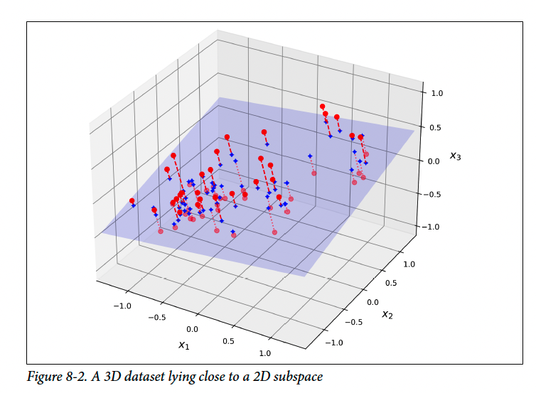
Projection works well when observations lie near a lower dimensional linear or affine subspace. For example, observations near a plane in three dimensional space can be projected onto that plane and represented using two new coordinates, $z_1$ and $z_2$.

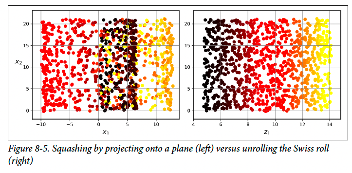
Projection may perform poorly when the underlying structure is curved. Projecting a Swiss roll directly onto a plane can collapse distinct layers and destroy important relationships.

Manifold Learning

Definition (Manifold).

A $d$ dimensional topological manifold is a space $M$ in which every point has a neighborhood that is homeomorphic to an open subset of $\mathbb{R}^d$. A smooth manifold additionally requires the coordinate transformations between overlapping neighborhoods to be differentiable.

Definition (Embedded manifold).

Let $M \subseteq \mathbb{R}^n$. The set $M$ is a $d$ dimensional embedded manifold if, for every point $p \in M$, there exists an open neighborhood $U \subseteq \mathbb{R}^n$ containing $p$ and a smooth invertible coordinate map $\phi: U \to V \subseteq \mathbb{R}^n$ with smooth inverse such that $\phi(U \cap M) = \{x \in V : x_{d+1} = \cdots = x_n = 0\}$. Thus, although $M$ may be globally curved inside $\mathbb{R}^n$, locally it has the structure of $\mathbb{R}^d$.

Remark (Embedded manifold).

A $d$ dimensional manifold embedded in $\mathbb{R}^n$, where $d < n$, is a subset that may be globally curved but locally resembles a $d$ dimensional plane.

Definition (Homeomorphism).

Let $X$ and $Y$ be topological spaces. A function $f: X \to Y$ is a homeomorphism if $f$ is bijective and continuous and its inverse $f^{-1}: Y \to X$ is also continuous. If such a function exists, $X$ and $Y$ are called homeomorphic, written $X \cong Y$. A homeomorphism preserves topological properties such as connectedness and continuity while allowing continuous stretching and bending.

Definition (Intrinsic dimension).

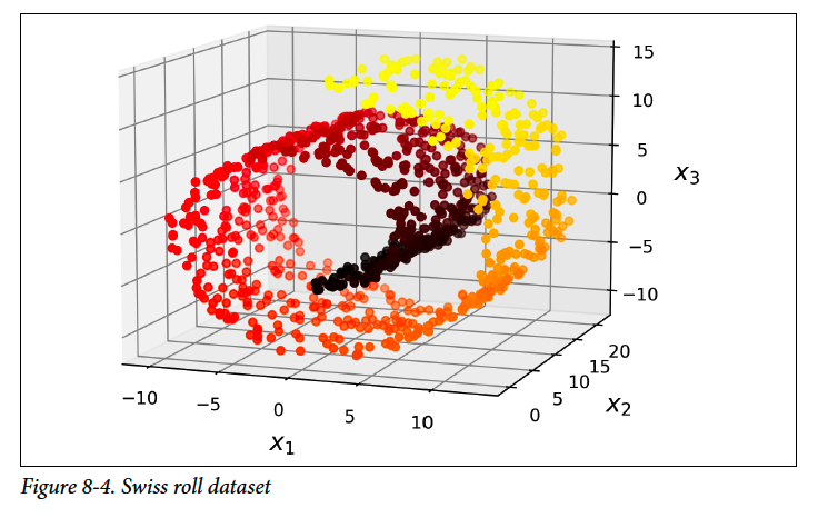
The intrinsic dimension is the number of independent coordinates needed to describe the data locally. A Swiss roll embedded in $\mathbb{R}^3$ has intrinsic dimension $2$ because two coordinates are sufficient to describe positions on its surface.

Definition (Manifold learning).

Let $\mathbf{x}_1,\ldots,\mathbf{x}_m \in \mathbb{R}^n$ be observations assumed to lie on or near a $d$ dimensional manifold $M \subseteq \mathbb{R}^n$, where $d \ll n$. Manifold learning seeks a mapping $f:M \to \mathbb{R}^d$ that assigns each observation $\mathbf{x}_i$ a lower dimensional representation $\mathbf{z}_i=f(\mathbf{x}_i)$ while approximately preserving relevant geometric or neighborhood structure of $M$. For methods that preserve distances, this may be expressed as $d_M(\mathbf{x}_i,\mathbf{x}_j) \approx \|\mathbf{z}_i-\mathbf{z}_j\|$, where $d_M$ denotes an appropriate distance measured along the manifold.

Remark (Manifold learning).

Manifold learning estimates the lower dimensional manifold on or near which observations lie and maps the observations to coordinates that preserve its meaningful structure.

The manifold hypothesis states that many real world datasets occupy a much lower dimensional manifold within their observed feature space. For example, valid handwritten digit images represent only a small fraction of all possible pixel combinations.

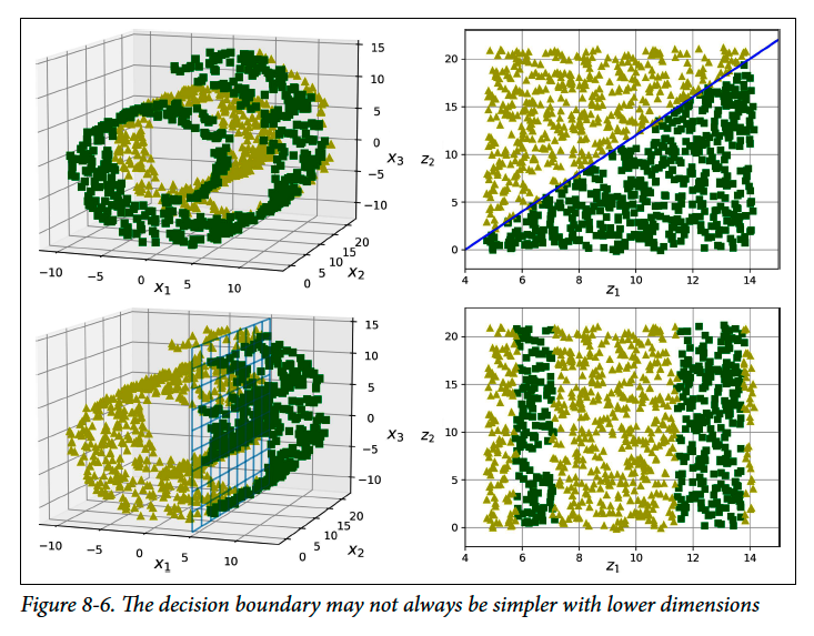
Unrolling a Swiss roll preserves its surface structure better than projecting it onto a plane. However, dimensionality reduction does not guarantee a simpler learning problem. A decision boundary that is complicated in the original space may become simple on the manifold, but the reverse can also occur.

Principal Component Analysis

Principal component analysis, or PCA, reduces dimensionality by finding a lower dimensional subspace that lies as close as possible to the data, then projecting the data onto that subspace.

Preserving Variance

PCA selects the projection axis that preserves the greatest amount of variance. This retains more information than projecting onto an axis with little variance.

==The axis that maximizes projected variance also minimizes the mean squared distance between the original observations and their projections.==

Principal Components

Definition (Principal component).

The $i$th principal component is the unit vector $c_i$ defining the direction that captures the greatest remaining variance, subject to being orthogonal to all preceding principal components.

The first principal component, $c_1$, captures the greatest variance. The second component, $c_2$, captures the greatest remaining variance while satisfying $c_1^\top c_2 = 0$.

For $n$ dimensional data, PCA can identify up to $n$ mutually orthogonal principal components.

Definition (Unit vector).

A unit vector is a vector whose Euclidean length is $1$. Formally, $c$ is a unit vector if $\|c\|_2 = \sqrt{c^\top c} = 1$.

Definition (Orthogonal vectors).

Two vectors $c_i$ and $c_j$ are orthogonal if their inner product is zero: $c_i^\top c_j = 0$.

The signs of principal component vectors are not stable. The vectors $c_i$ and $−c_i$ point in opposite directions but define the same axis. Small changes to the data may therefore reverse a component’s direction without changing the principal axis.

When two components capture very similar amounts of variance, they may rotate or exchange positions after small changes to the data. However, the subspace they collectively define generally remains stable.

Singular Value Decomposition

Definition (Singular value decomposition).

For any real matrix $X \in \mathbb{R}^{m \times n}$, a singular value decomposition is a factorization $X = U\Sigma V^\top$, where $U \in \mathbb{R}^{m \times m}$ and $V \in \mathbb{R}^{n \times n}$ are orthogonal matrices, and $\Sigma \in \mathbb{R}^{m \times n}$ is a rectangular diagonal matrix containing nonnegative singular values $\sigma_1 \geq \sigma_2 \geq \cdots \geq 0$.

An orthogonal matrix satisfies $U^\top U = I$ or $V^\top V = I$. Therefore, its columns form an orthonormal basis.

The columns of $V$ are the right singular vectors of $X$. When SVD is applied to a centered dataset, these vectors define the principal component directions. Equivalently, the rows of $V^\top$ contain the principal component vectors.

The singular values measure how much variation exists along their corresponding directions. For a centered dataset with $m$ observations, the variance captured by component $j$ is $\sigma_j^2/(m − 1)$.

The principal component matrix is $V = [c_1\ c_2\ \cdots\ c_n]$.

Computing Principal Components

import numpy as np

X = [...]  # create a small 3D dataset
X_centered = X - X.mean(axis=0)

U, s, Vt = np.linalg.svd(X_centered)

c1 = Vt[0]
c2 = Vt[1]

X_centered is created by subtracting each feature’s mean so that the dataset is centered around the origin.

Vt[0] contains the first principal component, while Vt[1] contains the second principal component. The array s contains the singular values in decreasing order.

PCA requires centered data. Scikit Learn’s PCA classes center the data automatically, but manual SVD requires centering before decomposition.

Projecting Down to $d$ Dimensions

After identifying the principal components, PCA reduces the dataset to $d$ dimensions by projecting it onto the hyperplane formed by the first $d$ principal components. These components preserve as much variance as possible.

If $W_d$ contains the first $d$ columns of $V$, the reduced dataset is calculated as $X_{d\text{ proj}}=XW_d$.

W2 = Vt[:2].T
X2D = X_centered @ W2

Using Scikit Learn

Scikit Learn uses SVD to perform PCA and automatically centers the data before applying the transformation.

from sklearn.decomposition import PCA

pca = PCA(n_components=2)
X2D = pca.fit_transform(X)

After fitting, components_ contains one row for each selected principal component. It corresponds to the transpose of $W_d$.

Explained Variance Ratio

The explained variance ratio measures the proportion of the dataset’s total variance captured by each principal component.

pca.explained_variance_ratio_

array([0.7578477, 0.15186921])

The first principal component captures approximately $76\%$ of the variance, while the second captures approximately $15\%$. Together, they preserve about $91\%$ of the total variance.

Choosing the Number of Dimensions

A common approach is to select the smallest number of principal components that preserve a chosen amount of variance, such as $95\%$. For visualization, the data is usually reduced to two or three dimensions instead.

from sklearn.datasets import fetch_openml

mnist = fetch_openml("mnist_784", as_frame=False)
X_train, y_train = mnist.data[:60_000], mnist.target[:60_000]
X_test, y_test = mnist.data[60_000:], mnist.target[60_000:]

pca = PCA()
pca.fit(X_train)

cumsum = np.cumsum(pca.explained_variance_ratio_)
d = np.argmax(cumsum >= 0.95) + 1

For MNIST, the minimum number of components required to preserve $95\%$ of the variance is $154$.

Scikit Learn can determine this number automatically by passing the desired variance ratio to n_components.

pca = PCA(n_components=0.95)
X_reduced = pca.fit_transform(X_train)

The selected number of components is stored in n_components_.

pca.n_components_

Another method is to plot cumulative explained variance against the number of dimensions. The elbow is the point where additional components provide much smaller increases in explained variance.

Choosing Dimensions for a Supervised Model

When PCA is used before a supervised model, the number of components can be treated as a hyperparameter and tuned together with the model.

from sklearn.ensemble import RandomForestClassifier
from sklearn.model_selection import RandomizedSearchCV
from sklearn.pipeline import make_pipeline

clf = make_pipeline(
    PCA(random_state=42),
    RandomForestClassifier(random_state=42)
)

param_distrib = {
    "pca__n_components": np.arange(10, 80),
    "randomforestclassifier__n_estimators": np.arange(50, 500)
}

rnd_search = RandomizedSearchCV(
    clf,
    param_distrib,
    n_iter=10,
    cv=3,
    random_state=42
)

rnd_search.fit(X_train[:1000], y_train[:1000])

{ "randomforestclassifier__n_estimators": 465, "pca__n_components": 23 }

The optimal number of components depends on the predictive model. In this example, the random forest performs best with only $23$ components. A linear model may require more components because it cannot learn patterns as flexibly.

PCA for Compression

PCA reduces storage by representing data with fewer principal component features. For MNIST, preserving $95\%$ of the variance reduces each observation from $784$ features to $154$ features, using less than $20\%$ of the original size.

The reduced data can be approximately reconstructed using the inverse transformation. For centered data, $X_{\text{recovered}}=X_{d\text{ proj}}W_d^\top$. Scikit Learn also restores the feature means automatically.

X_recovered = pca.inverse_transform(X_reduced)

The reconstruction is not exact because some variance was discarded. The mean squared distance between the original and reconstructed data is called the reconstruction error.

Randomized PCA

Randomized PCA approximates the first $d$ principal components using a stochastic algorithm. Its complexity is $O(md^2)+O(d^3)$, making it much faster than full SVD when $d$ is much smaller than $n$.

rnd_pca = PCA(
    n_components=154,
    svd_solver="randomized",
    random_state=42
)

X_reduced = rnd_pca.fit_transform(X_train)

With svd_solver="auto", Scikit Learn automatically chooses between randomized PCA and full SVD based on the dataset shape and requested number of components.

Incremental PCA

Incremental PCA processes the training set in batches, so the entire dataset does not need to fit in memory. Each batch is passed to partial_fit().

from sklearn.decomposition import IncrementalPCA

n_batches = 100
inc_pca = IncrementalPCA(n_components=154)

for X_batch in np.array_split(X_train, n_batches):
    inc_pca.partial_fit(X_batch)

X_reduced = inc_pca.transform(X_train)

A memory mapped array stores a large array in a binary file and loads only the required portions into memory.

filename = "my_mnist.mmap"

X_mmap = np.memmap(
    filename,
    dtype="float32",
    mode="write",
    shape=X_train.shape
)

X_mmap[:] = X_train
X_mmap.flush()

The data type and shape must be specified when reopening the file because only raw binary values are stored.

X_mmap = np.memmap(
    filename,
    dtype="float32",
    mode="readonly"
).reshape(-1, 784)

batch_size = X_mmap.shape[0] // n_batches

inc_pca = IncrementalPCA(
    n_components=154,
    batch_size=batch_size
)

inc_pca.fit(X_mmap)

Random Projection

Random projection reduces dimensionality using a randomly generated linear transformation. It requires no training because the data values are not examined when creating the projection matrix.

Johnson Lindenstrauss Lemma

Definition (Johnson Lindenstrauss lemma).

Let $S\subseteq\mathbb{R}^n$ contain $m$ points, and let $0<\varepsilon<1$. There exists a mapping $f:S\rightarrow\mathbb{R}^d$, where $d=O(\ln(m)/\varepsilon^2)$, such that every pair $x,y\in S$ satisfies $(1-\varepsilon)\lVert x-y\rVert^2\leq\lVert f(x)-f(y)\rVert^2\leq(1+\varepsilon)\lVert x-y\rVert^2$. A suitably scaled random linear projection satisfies this condition for all pairs with high probability.

The sufficient target dimension used by Scikit Learn is $d\geq\frac{4\ln(m)}{\varepsilon^2/2-\varepsilon^3/3}$. It depends on the number of observations $m$ and the accepted distortion $\varepsilon$, but not on the original number of features $n$.

For $m=5{,}000$ and $\varepsilon=0.1$, the required dimension is approximately $7{,}300$.

from sklearn.random_projection import (
    johnson_lindenstrauss_min_dim
)

m, ε = 5_000, 0.1
d = johnson_lindenstrauss_min_dim(m, eps=ε)

#d = 7300

Gaussian Random Projection

A Gaussian projection matrix $P$ has shape $(d,n)$, with each entry sampled from $\mathcal{N}(0,1/d)$. Dividing standard normal values by $\sqrt d$ produces the required variance.

n = 20_000
np.random.seed(42)

P = np.random.randn(d, n) / np.sqrt(d)

X = np.random.randn(m, n)
X_reduced = X @ P.T

The transformation changes the dataset from shape $(m,n)$ to $(m,d)$. Scikit Learn can determine $d$ from $\varepsilon$, generate the matrix, store it in components_, and apply the projection.

from sklearn.random_projection import (
    GaussianRandomProjection
)

gaussian_rnd_proj = GaussianRandomProjection(
    eps=ε,
    random_state=42
)

X_reduced = gaussian_rnd_proj.fit_transform(X)

Sparse Random Projection

SparseRandomProjection uses a sparse matrix instead of a dense Gaussian matrix. It usually requires much less memory and is faster, especially for large or sparse datasets, while providing comparable distance preservation.

Its default density is $r=1/\sqrt n$. Each matrix entry is nonzero with probability $r$, and a nonzero entry is either $-v$ or $+v$, where $v=1/\sqrt{dr}$.

Approximate Inverse Transformation

Random projection does not provide a direct inverse. An approximate reconstruction can be obtained using the pseudoinverse of the projection matrix.

components_pinv = np.linalg.pinv(
    gaussian_rnd_proj.components_
)

X_recovered = X_reduced @ components_pinv.T

Computing the pseudoinverse can be expensive for a large projection matrix. Random projection is therefore mainly useful for fast and memory efficient dimensionality reduction rather than accurate reconstruction.

Locally Linear Embedding

Locally linear embedding, or LLE, is a nonlinear dimensionality reduction and manifold learning technique. Unlike PCA and random projection, it does not project data onto learned axes. It preserves local relationships by reconstructing each observation from its nearest neighbors and then reproducing those relationships in a lower dimensional space.

from sklearn.datasets import make_swiss_roll
from sklearn.manifold import LocallyLinearEmbedding

X_swiss, t = make_swiss_roll(
    n_samples=1000,
    noise=0.2,
    random_state=42
)

lle = LocallyLinearEmbedding(
    n_components=2,
    n_neighbors=10,
    random_state=42
)

X_unrolled = lle.fit_transform(X_swiss)

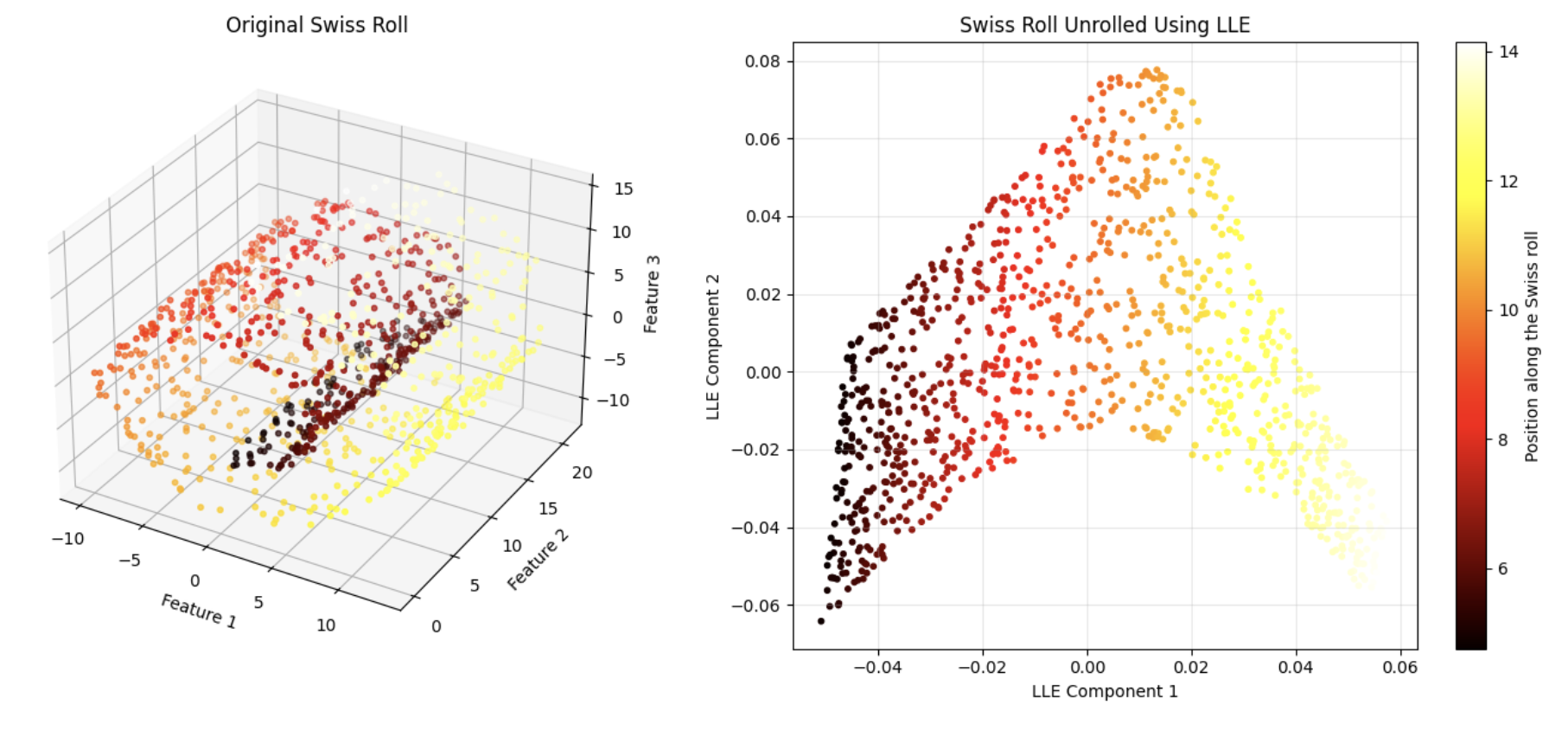
X_swiss has shape $(1000,3)$, while X_unrolled has shape $(1000,2)$. The variable t contains each observation’s position along the rolled axis and can be used as a regression target or for coloring the visualization.

LLE preserves distances and relationships locally, but it does not necessarily preserve large scale distances or the overall global shape.

Step 1: Constrained Optimization

For every observation $x^{(i)}$, LLE identifies its $k$ nearest neighbors and finds weights $w_{i,j}$ that reconstruct $x^{(i)}$ as accurately as possible.

$$\widehat{W} = \underset{W}{\operatorname{argmin}} \sum_{i=1}^{m} \left\| x^{(i)} - \sum_{j=1}^{m}w_{i,j}x^{(j)} \right\|_2^2 \quad \text{subject to} \quad \begin{cases} w_{i,j}=0, & x^{(j)}\notin\mathcal{N}_k(x^{(i)}) \\ \sum_{j=1}^{m}w_{i,j}=1, & i=1,\ldots,m \end{cases}$$

Here, $\mathcal{N}_k(x^{(i)})$ is the set of the $k$ nearest neighbors of $x^{(i)}$. The first constraint ensures that only neighbors contribute. The second normalizes the weights so they sum to $1$.

The resulting matrix $\widehat W$ encodes the local linear relationships among the original observations.

Step 2: Unconstrained Optimization

LLE keeps the learned weights fixed and finds lower dimensional coordinates $z^{(i)}$ that preserve the same reconstruction relationships.

$$\widehat{Z} = \underset{Z}{\operatorname{argmin}} \sum_{i=1}^{m} \left\| z^{(i)} - \sum_{j=1}^{m}\widehat{w}_{i,j}z^{(j)} \right\|_2^2$$

The matrix $Z$ contains all lower dimensional observations. Row $i$ of $Z$ is the new representation $z^{(i)}$ corresponding to $x^{(i)}$.

Although the book calls this unconstrained optimization, a completely unconstrained problem permits the trivial solution $Z=0$. Practical LLE removes this ambiguity using centering and scale conditions such as $Z^\top\mathbf{1}=0$ and $Z^\top Z=I$.

LLE obtains $Z$ by forming $M=(I-\widehat W)^\top(I-\widehat W)$ and using the eigenvectors associated with its smallest nonzero eigenvalues.

Computational Complexity

The approximate costs are $O(m\log(m)n\log(k))$ for finding neighbors, $O(mnk^3)$ for optimizing the weights, and $O(dm^2)$ for constructing the lower dimensional representation. The $m^2$ term causes LLE to scale poorly to very large datasets.

Other Dimensionality Reduction Techniques

Multidimensional Scaling

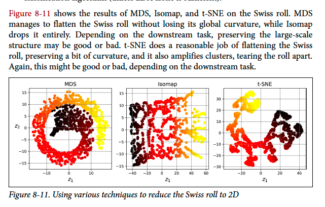
sklearn.manifold.MDS reduces dimensionality while attempting to preserve pairwise distances. It works better when the original data is not extremely high dimensional.

Isomap

sklearn.manifold.Isomap connects each observation to its nearest neighbors and creates a graph. It preserves geodesic distance, which is the shortest path distance between two graph nodes.

t-SNE

sklearn.manifold.TSNE attempts to keep similar observations close and dissimilar observations apart. It is mainly used to visualize clusters in two or three dimensions.

Linear Discriminant Analysis

sklearn.discriminant_analysis.LinearDiscriminantAnalysis is a supervised classification technique that learns axes that separate classes as much as possible. These axes can also be used for dimensionality reduction before classification.