Training Models

We focus our attention at the linear regression model. There are two ways to train it:

• Using a “closed-form” equation1 that directly computes the model parameters that best fit the model to the training set.
• Using an iterative optimization approach called gradient descent (GD) that gradually tweaks the model parameters to minimize the cost function over the training set, eventually converging to the same set of parameters as the first method.

A linear model makes a prediction by simply computing a weighted sum of the input features, plus a constant called the bias term (also called the intercept term), given by

$$\hat{y} = \theta_0 + \theta_1 x_1 +\theta_2 x_2 + \cdots + \theta_n x_n. \qquad\text{(1)}$$

where

• $\hat{y}$ is the predicted value
• $n$ is the number of features.
• $x_i$ is the ith feature value
• $\theta_j$ is the jth model parameter, including the bias term $\theta_0$ and the feature weights $\theta_i, i \in \mathbb{N}$

We can write the equation as

$$\hat{y} = h_{\mathbf{\theta}}(\mathbf{x}) = \mathbf{\theta} \cdot \mathbf{x} \qquad\text{(2)}$$

In this equation:

• $h_{\theta}$ is the hypothesis function, using the model parameters $\theta$.
• $\boldsymbol{\theta}$ is the model’s parameter vector, containing the bias term $\theta_{0}$ and the feature weights $\theta_{1}$ to $\theta_{n}$.
• $\mathbf{x}$ is the instance’s feature vector, containing $x_{0}$ to $x_{n}$, with $x_{0}$ always equal to $1$.
• $\boldsymbol{\theta} \cdot \mathbf{x}$ is the dot product of the vectors $\boldsymbol{\theta}$ and $\mathbf{x}$, which is equal to $\theta_{0}x_{0} + \theta_{1}x_{1} + \theta_{2}x_{2} + \dots + \theta_{n}x_{n}$.

Remark. Remark Learning algorithms often optimize a different loss function during training than the performance measure used for the final model evaluation. This is typically because the training loss is easier to optimize or includes extra terms (e.g., for regularization). A good performance metric should align closely with the final business objective, while a good training loss should be easy to optimize and strongly correlated with that metric. For example, classifiers may minimize log loss during training but evaluate performance with precision/recall

The MSE of a linear regression hypothesis $h_{\theta}$ on a training set $\mathbf{X}$ is calculated using

$$MSE(\mathbf{X}, h_{\theta}) = \frac{1}{m} \sum_{i=1}^m (\mathbf{\theta}^{\top} \mathbf{x}^i - y^i)^2$$

Theorem. The Normal Equation The value of $\theta$ that minimizes the MSE is given by

$$\hat{\mathbf{\theta}} = (\mathbf{X}^{\top}\mathbf{X})^{-1}\mathbf{X}^{\top} \mathbf{y}$$

where $\hat{\mathbf{\theta}}$ is the value of $\mathbf{\theta}$ that minimizes the cost function and $\mathbf{y}$ is the vector of target values containing $y^1$ to $y^m$.

Tip. add_dummy_feauture The add_dummy_feature function from sklearn.preprocessing adds an additional constant feature (usually set to 1) as the first column of the input array. This is often used to represent the bias term ($x_0 = 1$) in linear models, allowing the model to learn an intercept.

In this example, it ensures that X_new includes the bias term before performing the dot product with theta_best for predictions.

X_new = np.array([[0], [2]])
X_new_b = add_dummy_feature(X_new) # add x0 = 1 to each instance
y_predict = X_new_b @ theta_best
y_predict

Linear Regression

We can perform linear regression using Scikit-Learn directly.

from sklearn.linear_model import LinearRegression

lin_reg = LinearRegression()
lin_reg.fit(X, y)
lin_reg.intercept_, lin_reg.coef_

Scikit-Learn’s LinearRegression separates the intercept term (intercept_) from the feature weights (coef_). Internally, it relies on scipy.linalg.lstsq to solve the least squares problem. This can be called directly to compute parameters without explicitly using the model class.

The solution can also be obtained by computing the pseudoinverse (X⁺) of the feature matrix and multiplying it by the target vector (y). This pseudoinverse, also known as the Moore–Penrose inverse, can be computed using np.linalg.pinv().

The pseudoinverse is calculated using singular value decomposition (SVD), which factorizes the training matrix X into U Σ Vᵀ. The pseudoinverse is then V Σ⁺ Uᵀ, where small singular values are replaced with zero before inversion to improve numerical stability. This SVD-based approach is more robust than directly solving the Normal Equation, especially when XᵀX is singular or nearly singular.

from sklearn.linear_model import LinearRegression
lin_reg = LinearRegression()
lin_reg.fit(X, y)
lin_reg.intercept_, lin_reg.coef_
# (array([4.21509616]), array(2.77011339))
lin_reg.predict(X_new)
#array([[4.21509616],
       #[9.75532293]])

theta_best_svd, residuals, rank, s = np.linalg.lstsq(X_b, y, rcond=1e-6)
theta_best_svd
# array([[4.21509616],
       [#2.77011339]])

np.linalg.pinv(X_b) @ y
#array([[4.21509616],
       #[2.77011339]])

Note. > Both the Normal Equation and SVD become very slow with a large number of features (e.g., 100,000). However, they scale linearly with the number of training instances (O(m)), making them efficient for large datasets as long as they fit in memory.

Once a linear regression model is trained (using the Normal Equation or any other method), predictions are computationally fast. The complexity is linear with respect to both the number of prediction instances and the number of features. Doubling the number of instances or features roughly doubles prediction time.

Gradient Descent

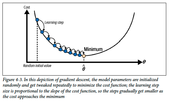
Definition. Gradient Descent Gradient descent is a generic optimization algorithm capable of finding optimal solutions to a wide range of problems. The general idea of gradient descent is to tweak parameters iteratively in order to minimize a cost function.

Gradient descent is similar to finding the steepest downhill path in dense fog. It measures the local gradient of the cost function with respect to parameters θ and moves in the direction of steepest descent until the gradient is zero (minimum). In practice, θ is randomly initialized, then updated step by step to reduce the cost (e.g., MSE) until convergence.

Warning. > An important parameter in gradient descent is the size of the steps, determined by the learning rate hyperparameter. If the learning rate is too small, then the algorithm will have to go through many iterations to converge, which will take a long time.

On the other hand, if the learning rate is too high, you might jump across the valley and end up on the other side, possibly even higher up than you were before. This might make the algorithm diverge, with larger and larger values, failing to find a good solution.

The MSE cost function for a linear regression model happens to be a convex function. This implies that there are no local minima, just one global minimum.

Remark. > The derivative of an MSE cost function is Lipschitz continuous. This and the convexity of MSE implies that the gradient descent is guaranteed to approach arbitrarily closely the global minimum.

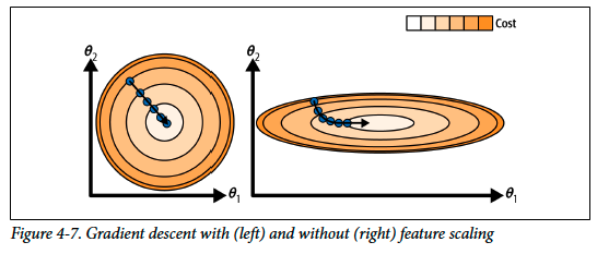
Tip. > When using gradient descent, you should ensure that all features have a similar scale (e.g., using Scikit-Learn’s StandardScaler class), or else it will take much longer to converge.

Batch Gradient Descent

Remark. Partial Derivative of MSE

$$\frac{\partial}{\partial \theta_j}MSE(\mathbf{\theta}) = \frac{2}{m} \sum_{i=1}^m (\mathbf{\theta}^{\top} \mathbf{x}^{(i)} - y^{(i)}x_j^{(i)}$$

Proof. Starting from the MSE cost function:

$$\begin{aligned} \text{MSE}(\boldsymbol{\theta}) &= \frac{1}{m} \sum_{i=1}^m \left( \boldsymbol{\theta}^T \mathbf{x}^{(i)} - y^{(i)} \right)^2, \\ \frac{\partial}{\partial \theta_j} \text{MSE}(\boldsymbol{\theta}) &= \frac{1}{m} \sum_{i=1}^m 2\left( \boldsymbol{\theta}^T \mathbf{x}^{(i)} - y^{(i)} \right) \cdot \frac{\partial}{\partial \theta_j}(\boldsymbol{\theta}^T \mathbf{x}^{(i)}), \\ &= \frac{2}{m} \sum_{i=1}^m \left( \boldsymbol{\theta}^T \mathbf{x}^{(i)} - y^{(i)} \right) x_j^{(i)}. \end{aligned}$$

Here, we note that

$$\boldsymbol{\theta}^T \mathbf{x}^{(i)} = \sum_{k=0}^n \theta_k x_k^{(i)} \Rightarrow \frac{\partial}{\partial \theta_j} \left( \boldsymbol{\theta}^T \mathbf{x}^{(i)} \right) = x_j^{(i)}$$

Thus

$$\frac{\partial}{\partial \theta_j} \text{MSE}(\boldsymbol{\theta}) = \frac{2}{m} \sum_{i=1}^m \left( \boldsymbol{\theta}^T \mathbf{x}^{(i)} - y^{(i)} \right) x_j^{(i)}.$$

□

Note that instead of doing these computations, we can use the gradient vector, $\nabla_{\theta} MSE(\mathbf{\theta})$.

$$\nabla_{\boldsymbol{\theta}} \text{MSE}(\boldsymbol{\theta}) = \begin{pmatrix} \frac{\partial}{\partial \theta_0} \text{MSE}(\boldsymbol{\theta}) \\ \frac{\partial}{\partial \theta_1} \text{MSE}(\boldsymbol{\theta}) \\ \vdots \\ \frac{\partial}{\partial \theta_n} \text{MSE}(\boldsymbol{\theta}) \end{pmatrix} = \frac{2}{m} \mathbf{X}^\top \left( \mathbf{X}\boldsymbol{\theta} - \mathbf{y} \right)$$

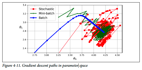
For convex cost functions with smooth slopes (e.g., MSE), batch gradient descent with a fixed learning rate will converge to the optimal solution, but it may take time. Convergence within tolerance ε requires about $O(1/\varepsilon)$ iterations. Increasing precision (e.g., dividing tolerance by 10) can make the algorithm run roughly 10× longer.

Stochastic Gradient Descent

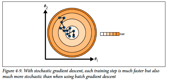
• Unlike batch gradient descent, which uses the whole training set per step, SGD updates parameters using one random training instance at a time.
• This makes it much faster and allows training on very large datasets, but updates are noisier, causing the cost to bounce around the minimum rather than settle exactly.
• The noise can help escape local minima, giving SGD a better chance of finding the global minimum in irregular cost functions.
• To balance exploration and convergence, the learning rate is gradually reduced over time (learning schedule).
• If reduced too quickly, the algorithm may get stuck; too slowly, it may bounce around and fail to converge.

Note. > For stochastic gradient descent to approach the global optimum, training instances must be independent and identically distributed (IID). This is typically ensured by shuffling instances randomly during training or at the start of each epoch. Without shuffling—such as when data is sorted by label—SGD may optimize for one label at a time and fail to converge near the global minimum.

To perform linear regression using stochastic GD with Scikit-Learn, you can use the SGDRegressor class, which defaults to optimizing the MSE cost function.

from sklearn.linear_model import SGDRegressor

sgd_reg = SGDRegressor(max_iter=1000, tol=1e-5, penalty=None, eta0=0.01, n_iter_no_change=100, random_state=42)
sgd_reg.fit(X, y.ravel())

This codes create an instance of the model with specific hyperparameters:

• max_iter=1000
  The maximum number of passes (epochs) over the training data. Here, up to 1000 iterations.

• tol=1e-5
  Tolerance for stopping criterion. Training stops early if the improvement in the loss function is smaller than 1e-5 for several iterations.

• penalty=None
  No regularization is applied. By default, SGDRegressor can use l2, l1, or elasticnet for regularization. Setting None means pure linear regression without regularization.

• eta0=0.01
  The initial learning rate for the gradient descent updates. Each step in SGD is scaled by this value.

• n_iter_no_change=100
  If the validation score does not improve for 100 consecutive iterations, training stops early. This prevents unnecessary computation if the model has already converged.

• random_state=42
  Ensures reproducibility by controlling randomization in the algorithm (important in SGD since data is shuffled each epoch).

• y.ravel() flattens the target y into a 1D array because SGDRegressor.fit() expects the target vector to be 1D (not a column vector).

  • Example: if y is shape (100, 1), .ravel() makes it (100,).

Tip. Tip Scikit-Learn estimators are usually trained with fit(), but some support partial_fit(), which trains incrementally on one or more instances without resetting parameters like max_iter or tol. This allows more control and gradual training. Some models also have warm_start=True, which lets fit() continue training from the previous state instead of resetting. Unlike fit(), which restarts the learning schedule counter, partial_fit() does not.

Definition. Learning Schedule A learning schedule (also called learning rate schedule) is a strategy that determines how the learning rate changes during training. T

• The learning rate (η or alpha) controls how big a step gradient descent takes when updating model parameters.
• If the learning rate is too high, the algorithm may overshoot and fail to converge.
• If it is too slow, convergence is very slow.

Mini-Batch Gradient Descent

Mini-batch GD computes gradients on small random subsets of the training set, combining the efficiency of batch GD and the speed of stochastic GD. It benefits from hardware optimizations (e.g., GPUs) and produces less erratic progress than stochastic GD.

With larger mini-batches, it converges closer to the minimum than stochastic GD, but may still wander around instead of settling. Batch GD stops at the minimum but is slower per step, while stochastic and mini-batch GD continue moving but still reach the minimum with a good learning schedule.

Polynomial Regression

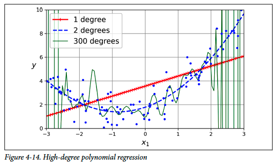
In polynomial regression, you can use a linear model to fit nonlinear data. A simple way to do this is to add powers of each feature as new features, then train a linear model on this extended set of features.

A quadratic dataset is generated with noise, showing that a linear model cannot capture its curvature. To solve this, PolynomialFeatures is used to add squared terms (degree=2) as new features. The transformed dataset (X_poly) contains both the original and squared features. A LinearRegression model is then fit to this extended dataset, producing a good fit for the quadratic trend.

from sklearn.preprocessing import PolynomialFeatures
poly_features = PolynomialFeatures(degree=2, include_bias=False)
X_poly = poly_features.fit_transform(X)
X[0] #array([-0.75275929])
X_poly[0] #array([-0.75275929,  0.56664654])

lin_reg = LinearRegression()
lin_reg.fit(X_poly, y)
lin_reg.intercept_, lin_reg.coef_
# (array([1.78134581]), array(0.93366893, 0.56456263))

Note. > PolynomialFeatures (degree=d) expands n features into $(n+d)! / (d! \times n!)$ features. This growth can be very large, so beware of the combinatorial explosion of features.

For example, with $d=2$ degree and $n=1$ feature (quadratic equation), it transforms into an array with $(2+1)!/(2\times 1)! = 3$ feaures.

Learning Curves

A high-degree polynomial regression model overfits training data, while a linear model underfits. The quadratic model generalizes best since the data was generated quadratically. To detect underfitting or overfitting, cross-validation is used: good training performance but poor cross-validation indicates overfitting; poor results on both indicate underfitting. Another method is examining learning curves, which plot training and validation error as functions of training set size.

Tip. Tip Scikit-Learn provides learning_curve(), which trains and evaluates models using cross-validation. By default, it retrains models on subsets of training data, but with exploit_incremental_learning=True, it can use incremental training (if supported with partial_fit() or warm_start). The function returns the training set sizes at which it evaluated the model, and the training and validation scores it measured for each size and for each cross-validation fold.

from sklearn.model_selection import learning_curve

train_sizes, train_scores, valid_scores = learning_curve(LinearRegression(), X, y, train_sizes=np.linspace(0.01, 1, 40), cv=5, scoring = 'neg_root_mean_squared_error')

train_scores = -train_scores.mean(axis=1)
valid_scores = -valid_scores.mean(axis=1)

The learning curves show an underfitting model. Training error starts at zero with very few instances but rises and plateaus as more data is added, since the model cannot perfectly fit noisy, nonlinear data. Validation error is initially high due to poor generalization, then decreases as more examples are shown, but also levels off near the training error. Both curves plateau close together, indicating the model is too simple to capture the data’s complexity.

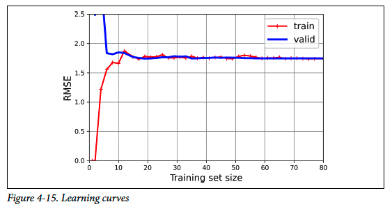
Note. Important The learning curves above are typical of a model that’s underfitting. Both curves have reached a plateau; they are close and fairly high.

Tip. > If your model is underfitting the training data, adding more training examples will not help. You need to use a better model or come up with better features.

The learning curves for a 10th-degree polynomial model differ from the underfitting case:

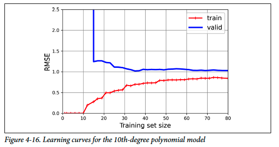
• Training error is much lower, showing the model fits the training data well.
• A noticeable gap exists between training and validation errors, indicating overfitting.

This gap is the hallmark of overfitting, as the model performs much better on training data than validation data. A way to reduce overfitting is to provide more training data, which helps bring validation error closer to training error.

The Bias/Variance Trade-Off

The Bias/Variance Trade-Off

• Bias: Error from wrong assumptions (e.g., assuming linear when data is quadratic). High bias leads to underfitting.
• Variance: Error from sensitivity to small variations. Complex models (e.g., high-degree polynomials) have high variance, leading to overfitting.
• Irreducible error: Error from inherent noise in the data, only reducible by improving data quality (e.g., fixing sensors, removing outliers).

Note. Important Increasing model complexity lowers bias but raises variance; reducing complexity lowers variance but raises bias. This trade-off explains the balance needed between underfitting and overfitting.

Regularized Linear Models

A good way to reduce overfitting is to regularize the model: the fewer degrees of freedom it has, the harder it will be for it to overfit the data. A simple way to regularize a polynomial model is to reduce the degree. For a linear model, we constrain the weights. We have three regularization methods:

• Ridge Regression
• Lasso Regression
• Elastic Net Regression

Ridge Regression (Tikhonov Regularization)

It is a regularized version of linear regression. No code is present in this section.

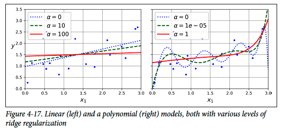
Ridge Regression (Tikhonov regularization) is a regularized form of linear regression where a penalty term $\frac{\alpha}{m}\sum_{i=1}^n \theta_i^2$is added to the MSE. This avoids large weights, helping prevent overfitting while still fitting the data. The penalty is only applied during training; model evaluation uses the unregularized MSE/RMSE.

$$J(\theta) = \text{MSE}(\theta) + \frac{\alpha}{m} \sum_{i=1}^n \theta_i^2$$

The hyperparameter $\alpha$ controls the strength of regularization:

• If $\alpha = 0$, ridge regression reduces to linear regression.
• If $\alpha$ is very large, weights shrink toward zero, and the model approaches a flat line at the data’s mean.

Here, we look at the $j$-th partial derivative of $J(\theta)$. Note that

$$\frac{\partial J(\theta)}{\partial \theta_j} = \frac{2}{m} \sum_{i=1}^{m} \big( \theta^\top x^{(i)} - y^{(i)} \big) x_j^{(i)} + \frac{2\alpha}{m} \theta_j$$

The extra term $\frac{2\alpha}{m} \theta_j$ does the following:

• This term pulls $\theta_j$ toward 0 during optimization.
• The larger $\alpha$, the stronger this pull.
• The optimizer minimizes the extra term by shrinking $\theta_j$ towards zero.

Note that we can write $\frac{\alpha}{m} \sum_{i=1}^n \theta_i^2$ as $\frac{\alpha}{m} ||\mathbf{w}||_2^2$ where $||w||_2$ represents the $\ell_2$ norm. For batch gradient descent, we just add $2\alpha \mathbf{w}/m$ to the part of the MSE gradient vector that correspond to the feature weights. That is,

$$\nabla_{\boldsymbol{\theta}} J(\boldsymbol{\theta}) = \begin{pmatrix} \frac{\partial J}{\partial \theta_0} \\ \frac{\partial J}{\partial \theta_1} \\ \vdots \\ \frac{\partial J}{\partial \theta_n} \end{pmatrix} = \underbrace{\frac{2}{m}\,\mathbf{X}^\top(\mathbf{X}\boldsymbol{\theta}-\mathbf{y})}_{\text{MSE gradient}} \;+\; \underbrace{\frac{2\alpha}{m} \begin{pmatrix} 0 \\ \theta_1 \\ \vdots \\ \theta_n \end{pmatrix}}_{\text{ridge penalty (bias not penalized)}}.$$

Warning. Warning It is important to scale the data (e.g., using a StandardScaler()) before performing ridge regression, as it is sensitive to the scale of the input features. This is true of most regularized models.

Remark. Ridge Regression Closed-form Solution

$$\hat{\mathbf{\theta}} = (\mathbf{X}^{\top} \mathbf{X} + \alpha \mathbf{A})^{-1}\mathbf{X}^{\top} \mathbf{y}$$

We can perform Ridge Regression using Scikit-Learn. We have the following.

from sklearn.linear_model import Ridge
ridge_reg = Ridge(alpha=0.1, solver="cholesky")
ridge_reg.fit(X, y)
ridge_reg.predict(1.5)

This is the variant of the closed-form solution which uses a factorization technique by Andre-Louis Cholesky.

Tip. RidgeCV The RidgeCV class performs ridge regression while automatically tuning hyperparameters using cross-validation. It is similar to GridSearchCV but optimized specifically for ridge regression, making it much faster. Other estimators also have cross-validation variants, such as LassoCV and ElasticNetCV.

Lasso Regression

Least absolute shrinkage and selection operator regression (lasso regression) is another regularized version of linear regression. The key difference of lasso regression from ridge regression is that it uses $\ell_2$ norm instead of $\ell_1$. The equation is given by

$$J(\mathbf{\theta})=MSE(\mathbf{\theta}) + 2\alpha \sum_{i=1}^n |{\theta_i}|$$

We notice the factor 2 in the equation. This is important to ensure that the optimal $\alpha$ is independent from the training set size: different norms lead to different factors.

• Lasso regression tends to eliminate less important features by setting their weights to zero. That is, lasso regression automatically performs feature selection and outputs a sparse model with few nonzero feature weights.
• This effectively performs feature selection and produces a sparse model with fewer nonzero weights.
• Example: with α = 0.01, polynomial feature weights shrink to zero, simplifying the model.

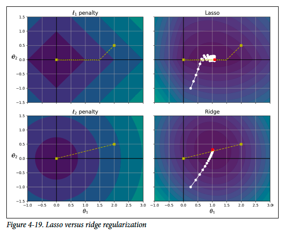
Figure 4-19 compares ℓ1 (Lasso) and ℓ2 (Ridge) penalties with contour plots of their loss functions.

• Top-left ($ℓ_1$ penalty): Contours represent $ℓ_1$ loss ($|θ_1| + |θ_2|$). Gradient descent reduces both parameters equally, but $θ_1$ tends to hit zero first. Gradients for $ℓ_1$ never reach 0 (either $-1$ or $1$ per parameter), so updates continue, causing bouncing near optimum.

• Top-right (Lasso): Contours represent Lasso’s cost (MSE + $ℓ_1$). Gradient descent shows $θ_2$ quickly reaching 0, then bouncing around the global optimum. Increasing $α$ shifts the optimum left; decreasing $α$ shifts it right. Lasso drives some weights exactly to zero, performing feature selection.

• Bottom-left ($ℓ_2$ penalty): Contours represent $ℓ_2$ loss. Gradient descent follows a straight path toward the origin since loss decreases smoothly as we move closer.

• Bottom-right (Ridge): Contours represent Ridge’s cost (MSE + $ℓ_2$). Gradients shrink near the optimum, so updates slow naturally, preventing bouncing. This makes Ridge converge faster than Lasso. With larger $α$, optimal parameters move closer to the origin but never exactly reach 0.

Highlighted point:

• "Which helps ridge converge faster than lasso regression."
• Ridge shrinks coefficients but does not eliminate them, unlike Lasso.

Note. > - Lasso ($ℓ_1$): Encourages sparsity by driving coefficients to exactly 0 (feature selection).

• Ridge ($ℓ_2$): Shrinks coefficients but keeps all features; converges more smoothly and faster.
• Increasing $α \to$ parameters move closer to the origin.

Tip. > To avoid bouncing around the optimum in Lasso regression, gradually reduce the learning rate during training. The model will still oscillate near the optimum, but with smaller and smaller steps, ensuring convergence.

The lasso cost function is not differentiable at $\theta_i = 0$ for $i = 1,2,\dots,n$.
However, gradient descent still works by using a subgradient vector $g(\theta, J)$.

The subgradient form is:

$$g(\theta, J) = \nabla_\theta \text{MSE}(\theta) + 2\alpha \begin{pmatrix} \text{sign}(\theta_1) \\ \text{sign}(\theta_2) \\ \vdots \\ \text{sign}(\theta_n) \end{pmatrix}$$

where

$$\text{sign}(\theta_i) = \begin{cases} -1 & \text{if } \theta_i < 0, \\ 0 & \text{if } \theta_i = 0, \\ +1 & \text{if } \theta_i > 0. \end{cases}$$

Here's the code, for example.

from sklearn.linear_model impor Lasso
lasso_reg = Lasso(alpha=0.1)
lasso_reg.fit(X,y)
lasso_reg.predict(1.5)
# array([1.53788174])

In this code, we can instead use SGDRegressor(penalty="l1", alpha=0.1).

Elastic Net Regression

Elastic Net regression is a middle ground between Ridge regression and Lasso regression. It uses a weighted sum of both Ridge’s ($\ell_2$) and Lasso’s ($\ell_1$) regularization terms, with a mix ratio $r$. That is, when $r=0$, it is equivalent to Ridge regression. When $r=1$, it is equivalent to Lasso regression. The equation is given below.

$$J(\theta) = \text{MSE}(\theta) + r \left(2 \alpha \sum_{i=1}^n |\theta_i|\right) + (1-r)\left(\frac{\alpha}{m} \sum_{i=1}^n \theta_i^2 \right)$$

Tip. > - Plain linear regression (no regularization) should generally be avoided.

• Ridge is a good default.
• Lasso or Elastic Net are preferred if only a few features are useful, since they push irrelevant feature weights to zero.
• Elastic Net is generally preferred over Lasso, as Lasso may behave erratically when the number of features is greater than the number of training instances or when features are strongly correlated.

from sklearn.linear_model import ElasticNet
elastic_net = ElasticNet(alpha=0.1, l1_ratio=0.5)
elastic_net.fit(X, y)
elastic_net.predict(1.5)
# array([1.54333232])

Early Stopping

A very different way to regularize iterative learning algorithms such as gradient descent is to stop training as soon as the validation error reaches a minimum. This is called early stopping.

• As training progresses, the training error (RMSE) decreases, and the validation error also goes down initially.
• After some epochs, the validation error stops decreasing and starts increasing again. This means the model has started to overfit the training data.
• With early stopping, you stop training as soon as the validation error reaches its lowest point.
• This is a simple and efficient regularization technique, famously described by Geoffrey Hinton as a “beautiful free lunch”.

Key Idea: Stop training at the epoch where validation error is minimized to avoid overfitting, even if training error continues to decrease.

Tip. > When using stochastic or mini-batch gradient descent, validation curves can be noisy, making it hard to spot the minimum. A common solution is to stop only after the validation error has stayed above the minimum for some time, then roll back the model parameters to the point where the validation error was lowest.

from copy import deepcopy
from sklearn.metrics import mean_squared_error
from sklearn.preprocessing import StandardScaler

# Data generation
np.random.seed(42)
m = 100
X = 6 * np.random.rand(m, 1) - 3
y = 0.5 * X ** 2 + X + 2 + np.random.randn(m, 1)

# Train/Validation split
X_train, y_train = X[: m // 2], y[: m // 2, 0] # this is the same with ravel
X_valid, y_valid = X[m // 2 :], y[m // 2 :, 0]

# Preprocessing pipeline
preprocessing = make_pipeline(PolynomialFeatures(degree=90, include_bias=False),
StandardScaler())
X_train_prep = preprocessing.fit_transform(X_train)
X_valid_prep = preprocessing.transform(X_valid)

# SGD regressor setup
sgd_reg = SGDRegressor(penalty=None, eta0=0.002, random_state=42)
n_epochs = 500
best_valid_rmse = float('inf')
train_errors, val_errors = [], []

# Training loop
for epoch in range(n_epochs): # allows incremental learning
	sgd_reg.partial_fit(X_train_prep, y_train)
	y_valid_predict = sgd_reg.predict(X_valid_prep)
	val_error = mean_squared_error(y_valid, y_valid_predict, squared=False)
	if val_error < best_valid_rmse:
		best_valid_rmse = val_error
		best_model = deepcopy(sgd_reg) # Saves the model if it’s the best so far.
		# extra code – we evaluate the train error and save it for the figure
		
    y_train_predict = sgd_reg.predict(X_train_prep)
    train_error = root_mean_squared_error(y_train, y_train_predict)
    val_errors.append(val_error)
    train_errors.append(train_error)

Note that in this code, deepcopy is used to store the best-performing model during training so it won’t be overwritten as the SGD updates continue. It copies both the model’s hyperparameters and the learned parameters.

Logistic Regression

Logistic regression (also called logit regression) is a regression algorithm often used for classification. It estimates the probability that an instance belongs to a class (positive class = 1, negative class = 0). If the probability is greater than a threshold (usually 50%), the model predicts class 1; otherwise, class 0. This makes it a binary classifier.

A logistic regression model works like linear regression, computing a weighted sum of inputs (plus bias). But instead of outputting the raw value, it applies the logistic (sigmoid) function to map the result between 0 and 1. The logistic regression model estimated probability is given by

$$\hat{p} = h_\theta(x) = \sigma(\theta^T x)$$

The logistic function $\sigma(\cdot)$ is given by

$$\sigma(t) = \frac{1}{1 + \exp(-t)}$$

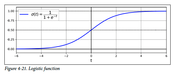
Once the probability $\hat{p}$ is estimated, the model predicts class $\hat{y}$ using a threshold of 0.5. Logistic regression model prediction using a 50% threshold probability:

$$\hat{y} = \begin{cases} 0 & \text{if } \hat{p} < 0.5 \\ 1 & \text{if } \hat{p} \geq 0.5 \end{cases}$$

• If $t < 0$, then $\sigma(t) < 0.5$, so prediction = 0.
• If $t \geq 0$, then $\sigma(t) \geq 0.5$, so prediction = 1.

Thus, the sign of $\theta^T x$ determines the class. If $\theta^T x > 0$, then $\sigma > 0$. Otherwise, $\sigma < 0$.

Note. > The score $t$ is called the logit, which is the inverse of the logistic function. The logit is defined as $\text{logit}(p) = \log\left(\frac{p}{1 - p}\right)$ and represents the log-odds (logarithm of the odd ratio), meaning it is the logarithm of the ratio between the probability of the positive class and that of the negative class. Computing the logit of an estimated probability $p$ returns the score $t$.

Remark. > The logistic (sigmoid) function $\sigma:\mathbb{R}\to(0,1)$ given by

$$\sigma(t) = \frac{1}{1+e^{-t}}$$

and the logit (log-odds) function $\operatorname{logit}:(0,1)\to\mathbb{R}$ given by

$$\operatorname{logit}(p) = \log\!\left(\frac{p}{1-p}\right)$$

are inverses of one another. That is, $\sigma(t) = p \Longleftrightarrow \text{logit}(p)=t$.

Proof. ($\Rightarrow$) Let $p=\sigma(t)=\dfrac{1}{1+e^{-t}}$ with $t\in\mathbb{R}$. Then

$$\frac{1}{p}=1+e^{-t}\Longrightarrow\frac{1-p}{p}=e^{-t} \Longrightarrow -\log\!\left(\frac{1-p}{p}\right)=t.$$

Hence

$$\operatorname{logit}(p)=\log\!\left(\frac{p}{1-p}\right)=t,$$

so $\operatorname{logit}(\sigma(t))=t$. ($\Leftarrow$) Let $z=\operatorname{logit}(p)=\log\!\left(\dfrac{p}{1-p}\right)$ with $p\in(0,1)$. Exponentiating gives

$$e^{z}=\frac{p}{1-p}\Longrightarrow p=\frac{e^{z}}{1+e^{z}} =\frac{1}{1+e^{-z}}=\sigma(z).$$

Thus $\sigma(\operatorname{logit}(p))=p$. □

Training Cost Function

The objective of training logistic regression is to set the parameter vector $\theta$ so that the model estimates high probabilities for positive instances ($y = 1$) and low probabilities for negative instances ($y = 0$).This is achieved using the cost function shown in the equation below.

$$c(\theta) = \begin{cases} -\log(\hat{p}) & \text{if } y = 1 \\ -\log(1 - \hat{p}) & \text{if } y = 0 \end{cases}$$

The function penalizes the model heavily when its estimated probability is close to the wrong outcome:

• If the true label is $y=1$:
  The cost is $-\log(\hat{p})$.
  • If $\hat{p} \approx 1$, then $\log(\hat{p}) \approx 0$ → cost is small (good).
  • If $\hat{p} \approx 0$, then $\log(\hat{p}) \to -\infty$ → cost is very large (bad).
• If the true label is $y=0$:
  The cost is $-\log(1-\hat{p})$.
  • If $\hat{p} \approx 0$, then $\log(1-\hat{p}) \approx 0$ → cost is small (good).
  • If $\hat{p} \approx 1$, then $\log(1-\hat{p}) \to -\infty$ → cost is very large (bad).

This behavior ensures that the model is trained to assign probabilities correctly for classification. The cost function for logistic regression over the entire training set is the average cost of all training instances. This is expressed in the equation below.

$$J(\theta) = -\frac{1}{m} \sum_{i=1}^m \left[ y^{(i)} \log \hat{p}^{(i)} + \left(1 - y^{(i)}\right) \log \left(1 - \hat{p}^{(i)}\right) \right]$$

This equation combines the individual costs: $-\log(\hat{p})$ when $y=1$, and $-\log(1-\hat{p})$ when $y=0$, into one unified formula. The log loss penalizes wrong predictions more heavily as they become more confident in the wrong direction, encouraging the model to estimate probabilities correctly.

Note. > The log loss is not arbitrary—it can be justified mathematically using Bayesian inference. Minimizing log loss corresponds to finding the model with the maximum likelihood of being optimal, under the assumption that data instances follow a Gaussian distribution around their class mean. When you use the log loss, this is the implicit assumption you are making. If this assumption is wrong, the model will be biased.

Thus, both log loss and MSE rely on statistical assumptions about the data, and when those assumptions fail, bias is introduced.

There is no closed-form equation to compute the value of $\mathbf{\theta}$ that minimizes the cost function. But this cost function is convex, so GD or other optimization algorithm is guaranteed to find the global minimum. The partial derivative is given by

$$\frac{\partial}{\partial \theta_j} J(\theta) = \frac{1}{m} \sum_{i=1}^m \left( \sigma(\theta^T x^{(i)}) - y^{(i)} \right) x_j^{(i)}$$

This looks very similar to the gradient equation in linear regression:

• For each instance, it computes the prediction error and multiplies it by the $j^{th}$ feature value.
• Then it averages the result across all training instances.
• These partial derivatives form the gradient vector, which can be used in batch gradient descent.

Decision Boundaries