Support Vector Machines

A support vector machine (SVM) is capable for linear/nonlinear classification and regression. They are only good for small to medium-sized nonlinear datasets and do not scale well to large datasets.

Large margin classification - the idea of choosing the widest possible “street” between classes so the classifier is more robust on new data.

Remark. Remark SVMs are sensitive to feature scales.

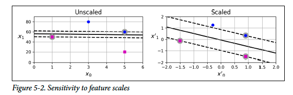
Hard margin classification - the idea of imposing that all instances must be on the correct side. This only works if data is linearly separable and this is sensitive to outliers. Soft margin classification - the balance between large margin classification and hard margin classification.

When creating SVM model, there is a hyperparameter C where increasing C makes the street smaller and reducing makes the street larger.

Remark. >If your SVM model is overfitting, you can try regularizing it by reducing C.

Although linear SVM classifiers are efficient and often work surprisingly well, many datasets are not even close to being linearly separable.

The kernel trick makes it possible to get the same result as if you had added many polynomial features, even with a very high degree, without actually having to add them.

Similarity Features

Similarity features are new features created by measuring how close each data point is to selected reference points called landmarks.

Instead of representing an instance only by its original feature value, we represent it by its similarity to one or more landmarks.

For example, suppose we have a one-dimensional point $x$ and a landmark $\ell$. We can measure their similarity using the Gaussian RBF similarity function:

$$\phi_\gamma(x, \ell) = \exp(-\gamma \|x - \ell\|^2)$$

where:

• $x$ is the data point
• $\ell$ is the landmark
• $\|x - \ell\|^2$ is the squared distance between them
• $\gamma$ controls how fast similarity decreases as distance increases

The output is always between $0$ and $1$:

• close to $1$ means the point is very similar or close to the landmark
• close to $0$ means the point is far from the landmark

The key idea is that similarity features can transform a nonlinear dataset into a higher-dimensional feature space where it may become linearly separable. This allows a linear model, such as a linear SVM, to solve problems that were not linearly separable in the original feature space.

Support Vector Regression (SVR)

Support Vector Regression (SVR) is an extension of Support Vector Machines used for regression tasks. Instead of trying to separate classes with the widest possible margin, SVR tries to fit a function that keeps as many training instances as possible within a margin of width $\epsilon$ around the predicted regression line, while limiting the number and size of margin violations.

Formally, SVR seeks a function $f(x)$ such that most predictions satisfy

$$|y_i - f(x_i)| \leq \epsilon$$

where $\epsilon$ defines the width of the margin, also called the $\epsilon$-insensitive tube. Errors inside this tube are ignored, meaning that training instances within the margin do not affect the model’s predictions. Only instances outside the tube contribute to the loss and become support vectors.

A smaller value of $\epsilon$ creates a narrower margin, which usually increases the number of support vectors and makes the model more sensitive to the training data. A larger value of $\epsilon$ creates a wider margin, allowing more instances to fall inside the tube and producing a simpler, smoother model.

Theorem. Distance Between Parallel Hyperplanes Let $\mathbf{w} \in \mathbb{R}^n$ with $\mathbf{w} \neq \mathbf{0}$, and let $b,c_1,c_2 \in \mathbb{R}$. Consider the parallel hyperplanes $H_1=\{\mathbf{x}:\mathbf{w}^T\mathbf{x}+b=c_1\}$ and $H_2=\{\mathbf{x}:\mathbf{w}^T\mathbf{x}+b=c_2\}$. Then the distance between them is

$$d(H_1,H_2)=\frac{|c_2-c_1|}{\|\mathbf{w}\|}.$$

Proof. Let $\mathbf{x}_1 \in H_1$, so $\mathbf{w}^T\mathbf{x}_1+b=c_1$. Since $\mathbf{w}$ is normal to both hyperplanes, the shortest path from $H_1$ to $H_2$ is in the direction of the unit normal vector $\frac{\mathbf{w}}{\|\mathbf{w}\|}$. Thus, a point on $H_2$ can be written as $\mathbf{x}_2=\mathbf{x}_1+\alpha\frac{\mathbf{w}}{\|\mathbf{w}\|}$, where $|\alpha|$ is the distance traveled. Since $\mathbf{x}_2 \in H_2$, we have $\mathbf{w}^T\mathbf{x}_2+b=c_2$. Substituting $\mathbf{x}_2$ gives $\mathbf{w}^T\left(\mathbf{x}_1+\alpha\frac{\mathbf{w}}{\|\mathbf{w}\|}\right)+b=c_2$. Hence, $\mathbf{w}^T\mathbf{x}_1+b+\alpha\frac{\mathbf{w}^T\mathbf{w}}{\|\mathbf{w}\|}=c_2$. Since $\mathbf{w}^T\mathbf{x}_1+b=c_1$ and $\mathbf{w}^T\mathbf{w}=\|\mathbf{w}\|^2$, we get $c_1+\alpha\|\mathbf{w}\|=c_2$. Therefore, $\alpha=\frac{c_2-c_1}{\|\mathbf{w}\|}$. Taking the absolute value gives $d(H_1,H_2)=|\alpha|=\frac{|c_2-c_1|}{\|\mathbf{w}\|}$. □

Definition. Hard-Margin Linear SVM Objective The hard-margin linear SVM classifier finds the weight vector $\mathbf{w}$ and bias term $b$ that maximize the margin while ensuring that every training instance is correctly classified and lies outside the margin. This can be written as the constrained optimization problem:

$$\min_{\mathbf{w},b}\frac{1}{2}\mathbf{w}^T\mathbf{w}$$

subject to

$$t^{(i)}(\mathbf{w}^T\mathbf{x}^{(i)}+b)\geq 1 \quad \text{for } i=1,2,\dots,m.$$

Here, $\mathbf{w}$ is the weight vector, $b$ is the bias term, $\mathbf{x}^{(i)}$ is the $i$-th training instance, and $t^{(i)}$ is the transformed class label, where $t^{(i)}=-1$ for the negative class and $t^{(i)}=1$ for the positive class.

The constraint $t^{(i)}(\mathbf{w}^T\mathbf{x}^{(i)}+b)\geq 1$ ensures that all training instances are correctly classified and lie outside the margin. For positive instances, this means $\mathbf{w}^T\mathbf{x}^{(i)}+b\geq 1$. For negative instances, this means $\mathbf{w}^T\mathbf{x}^{(i)}+b\leq -1$.

We minimize $\frac{1}{2}\mathbf{w}^T\mathbf{w}$ instead of directly maximizing the margin because the margin width is $\frac{2}{\|\mathbf{w}\|}$. Thus, maximizing the margin is equivalent to minimizing $\|\mathbf{w}\|$. The expression $\frac{1}{2}\mathbf{w}^T\mathbf{w}=\frac{1}{2}\|\mathbf{w}\|^2$ is preferred because it is differentiable and easier to optimize. The factor $\frac{1}{2}$ is included for convenience, since its derivative is simply $\mathbf{w}$.

Definition. Soft-Margin Linear SVM Objective The soft-margin linear SVM introduces a slack variable $\zeta^{(i)} \geq 0$ for each training instance. The value of $\zeta^{(i)}$ measures how much the $i$-th instance is allowed to violate the margin. The objective is to keep the margin as wide as possible while allowing some margin violations.

The soft-margin linear SVM objective is written as:

$$\min_{\mathbf{w},b,\zeta}\frac{1}{2}\mathbf{w}^T\mathbf{w}+C\sum_{i=1}^{m}\zeta^{(i)}$$

subject to

$$t^{(i)}(\mathbf{w}^T\mathbf{x}^{(i)}+b)\geq 1-\zeta^{(i)} \quad \text{and} \quad \zeta^{(i)}\geq 0 \quad \text{for } i=1,2,\dots,m.$$

Here, $\frac{1}{2}\mathbf{w}^T\mathbf{w}$ encourages a wider margin, while $\sum_{i=1}^{m}\zeta^{(i)}$ penalizes margin violations. The hyperparameter $C$ controls the trade-off between these two goals. A larger $C$ penalizes margin violations more strongly, leading to fewer violations but possibly a narrower margin. A smaller $C$ allows more violations, giving a wider and more regularized margin.

Both hard-margin and soft-margin SVMs are convex quadratic optimization problems with linear constraints, also called quadratic programming (QP) problems.

The Dual Problem

Definition. The Dual Problem Given a constrained optimization problem called the primal problem, it is often possible to express a closely related problem called the dual problem. Under certain conditions, such as those satisfied by SVM optimization, the primal and dual problems have the same solution. This means we can solve either the primal or the dual formulation.

For the linear SVM, the dual objective can be written as:

$$\min_{\boldsymbol{\alpha}} \frac{1}{2}\sum_{i=1}^{m}\sum_{j=1}^{m}\alpha^{(i)}\alpha^{(j)}t^{(i)}t^{(j)}{\mathbf{x}^{(i)}}^T\mathbf{x}^{(j)}-\sum_{i=1}^{m}\alpha^{(i)}$$

subject to

$$\alpha^{(i)} \geq 0 \quad \text{for all } i=1,2,\dots,m \quad \text{and} \quad \sum_{i=1}^{m}\alpha^{(i)}t^{(i)}=0.$$

Here, $\alpha^{(i)}$ are the dual variables, $t^{(i)}$ are the transformed labels where $t^{(i)}\in\{-1,1\}$, and ${\mathbf{x}^{(i)}}^T\mathbf{x}^{(j)}$ is the dot product between two training instances.

Once the optimal dual variables $\hat{\boldsymbol{\alpha}}$ are found, we can recover the primal solution using:

$$\hat{\mathbf{w}}=\sum_{i=1}^{m}\hat{\alpha}^{(i)}t^{(i)}\mathbf{x}^{(i)}$$

and

$$\hat{b}=\frac{1}{n_s}\sum_{\substack{i=1 \\ \hat{\alpha}^{(i)}>0}}^{m}\left(t^{(i)}-\hat{\mathbf{w}}^T\mathbf{x}^{(i)}\right),$$

where $n_s$ is the number of support vectors.

The dual problem is often faster to solve than the primal problem when the number of training instances is smaller than the number of features. More importantly, the dual formulation makes the kernel trick possible, because the data only appears through dot products ${\mathbf{x}^{(i)}}^T\mathbf{x}^{(j)}$.

Theorem. Mercer's Theorem Let $\mathcal{X}$ be a compact subset of $\mathbb{R}^n$, and let $K:\mathcal{X}\times\mathcal{X}\to\mathbb{R}$ be a continuous, symmetric function. If $K$ is positive semidefinite, meaning that for any finite set $\mathbf{x}^{(1)},\dots,\mathbf{x}^{(m)}\in\mathcal{X}$ and any real coefficients $c_1,\dots,c_m$, we have

$$\sum_{i=1}^{m}\sum_{j=1}^{m}c_i c_j K(\mathbf{x}^{(i)},\mathbf{x}^{(j)})\geq 0,$$

then there exists a Hilbert space $\mathcal{H}$ and a feature map $\phi:\mathcal{X}\to\mathcal{H}$ such that

$$K(\mathbf{a},\mathbf{b})=\langle \phi(\mathbf{a}),\phi(\mathbf{b})\rangle_{\mathcal{H}}.$$

In SVMs, this means that if a function $K$ satisfies Mercer's conditions, then it can be used as a valid kernel function. The kernel computes an inner product in some transformed feature space without explicitly computing the transformation $\phi$. This is what makes the kernel trick possible.

For example, the Gaussian RBF kernel is given by

$$K(\mathbf{a},\mathbf{b})=\exp(-\gamma\|\mathbf{a}-\mathbf{b}\|^2).$$

This kernel corresponds to an inner product in a very high-dimensional, even infinite-dimensional, feature space. Mercer's theorem guarantees that such a feature map $\phi$ exists, even if we do not explicitly write it down.

Note. > Some kernels used in practice, such as the sigmoid kernel, do not always satisfy all of Mercer's conditions, but they may still work well empirically.