Unsupervised Learning Techniques
Clustering, anomaly detection, density estimation, K-means, DBSCAN, and other techniques for learning patterns from unlabeled data.
Most available data is unlabeled data, meaning the input features are available but the target labels are not. Unsupervised learning allows algorithms to discover useful structures and patterns directly from this unlabeled data.
Main Unsupervised Learning Tasks
Clustering
Clustering groups similar instances into clusters. Unlike classification, the correct group labels are not provided beforehand. The algorithm must discover the groups based on similarities within the data.
Anomaly Detection
Anomaly detection, also called outlier detection, learns what normal data looks like and identifies unusual instances called anomalies or outliers. Applications include fraud detection, detecting manufacturing defects, identifying unusual time series patterns, and removing outliers before model training.
Density Estimation
Density estimation estimates the probability density function of the process that generated the data. Regions with very low density may contain anomalies. Density estimation is also useful for data analysis and visualization.
Clustering Algorithms
This chapter focuses primarily on K means and DBSCAN. Gaussian mixture models are later introduced for density estimation, clustering, and anomaly detection.
A cluster is a group of similar instances. There is no universal definition of what a cluster should look like. Different clustering algorithms identify different kinds of structures. Some focus on instances around a central point called a centroid, while others identify continuous dense regions or hierarchical groups.
Applications of Clustering
Customer segmentation groups customers according to characteristics such as purchases and website activity. These groups can help businesses understand different customer needs, personalize marketing, and improve recommender systems.
Data analysis can use clustering to divide a dataset into meaningful groups so that each cluster can be analyzed separately.
Dimensionality reduction can represent an instance using its affinity to each cluster. If there are clusters, the original feature vector can be replaced by a vector containing cluster affinities, potentially reducing dimensionality.
Feature engineering can use cluster affinities as additional features. For example, geographic cluster affinities can provide useful information about location.
Anomaly detection can identify instances with low affinity to every cluster as potential anomalies.
Semi supervised learning can use clustering when only a few labels are available. Labels can be propagated from labeled instances to other instances in the same cluster, producing more labeled data for supervised learning.
Search engines can cluster similar items such as images. When a reference image is provided, the system can identify its cluster and retrieve similar instances from that cluster.
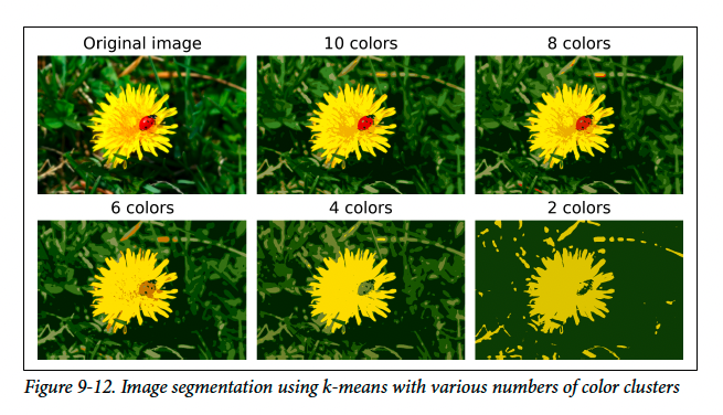
Image segmentation can cluster pixels according to properties such as color. Each pixel can then be replaced by the mean color of its cluster, reducing the number of colors and making object boundaries easier to detect.
K Means
K Means is an unsupervised clustering algorithm that groups instances into clusters. It finds a centroid for each cluster and assigns every instance to the cluster whose centroid is closest. The number of clusters must be specified beforehand.
from sklearn.cluster import KMeans
from sklearn.datasets import make_blobs

X, y = make_blobs([...])

k = 5
kmeans = KMeans(n_clusters=k, random_state=42)
y_pred = kmeans.fit_predict(X)
fit_predict(X)trains the K Means model and returns the cluster label assigned to every training instance.
Centroids
After training, the coordinates of the learned centroids are available through cluster_centers_.
kmeans.cluster_centers_
array([[-2.80389616,  1.80117999],
       [ 0.20876306,  2.25551336],
       [-2.79290307,  2.79641063],
       [-1.46679593,  2.28855348],
       [-2.80037642,  1.30082566]])
New instances can be assigned to their nearest centroid using predict().
import numpy as np

X_new = np.array([[0, 2], [3, 2], [-3, 3], [-3, 2.5]])
kmeans.predict(X_new)
Voronoi Tessellation
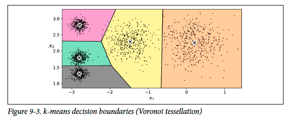
The decision boundaries produced by K Means form a Voronoi tessellation. Each region contains all locations that are closest to the same centroid.
K Means can assign some instances poorly when clusters have different sizes, densities, or shapes because the assignment depends on distance to the centroid.
Hard and Soft Clustering
Hard clustering assigns each instance to exactly one cluster. Soft clustering gives each instance a score for every cluster. The score may be based on distance to the centroid or a similarity measure such as the Gaussian radial basis function.
In Scikit Learn, transform() returns the distance from every instance to every centroid.
kmeans.transform(X_new).round(2)
array([[2.81, 0.33, 2.90, 1.49, 2.89],
       [5.81, 2.80, 5.85, 4.48, 5.84],
       [1.21, 3.29, 0.29, 1.69, 1.71],
       [0.73, 3.22, 0.36, 1.55, 1.22]])
If there are clusters, transforming the dataset this way produces distance features. These distances can be used for nonlinear dimensionality reduction or as extra features for another model.
The K Means Algorithm
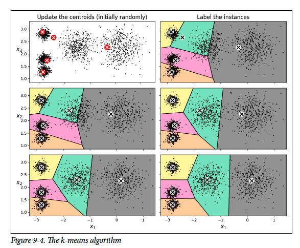
K Means repeatedly performs two main operations.
Assignment Step
Each instance is assigned to the cluster whose centroid is closest. For an instance , its assigned cluster can be written as , where represents centroid .
Centroid Update Step
Each centroid is recomputed as the mean of all instances assigned to that cluster. For cluster , the updated centroid is .
The process is:
initialize centroids → assign instances → update centroids → assign instances again → update centroids → repeat
Training stops when the centroids stop moving.
The algorithm is guaranteed to converge in a finite number of iterations because the mean squared distance between the instances and their closest centroids can only decrease or remain unchanged, and it cannot become negative.
Centroid Initialization
Poor initial centroid positions can cause K Means to converge to a suboptimal clustering. If approximate centroid locations are already known, they can be supplied through init.
good_init = np.array([
    [-3, 3],
    [-3, 2],
    [-3, 1],
    [-1, 2],
    [0, 2]
])

kmeans = KMeans(
    n_clusters=5,
    init=good_init,
    n_init=1,
    random_state=42
)

kmeans.fit(X)
initdetermines how the initial centroid locations are chosen.n_initdetermines how many different initializations are tried. K Means keeps the solution with the lowest inertia.
Inertia
Inertia is the sum of the squared distances between every instance and its closest centroid. It can be written as Lower inertia means that instances are collectively closer to their assigned centroids.
kmeans.inertia_
kmeans.score(X)
The score() method returns the negative inertia because Scikit Learn follows the convention that a larger score should represent a better model. When several initializations are tried, K Means keeps the model with the lowest inertia.
K-Means++
K Means Plus Plus improves centroid initialization by choosing starting centroids that tend to be far apart. This reduces the probability of converging to a poor local optimum.
The first centroid is selected uniformly at random from the dataset.
For every remaining instance , calculate , which is its distance to the closest centroid already selected.
The next centroid is selected with probability .
Therefore, instances that are farther away from the already selected centroids have a greater probability of becoming the next centroid. The process is repeated until all initial centroids have been selected.
K Means Plus Plus is the default initialization method used by KMeans.
Accelerated K-Means
The Elkan algorithm can accelerate K Means by avoiding unnecessary distance calculations. It uses the triangle inequality and keeps lower and upper bounds on distances between instances and centroids.
Its effectiveness depends on the dataset, and in some situations it may actually slow training.
Mini Batch K-Means
Mini Batch K Means processes small batches of instances instead of the full dataset during every iteration.
Each mini batch moves the centroids slightly. This reduces computation time and makes it possible to cluster datasets that do not fit entirely in memory.
from sklearn.cluster import MiniBatchKMeans

minibatch_kmeans = MiniBatchKMeans(
    n_clusters=5,
    random_state=42
)

minibatch_kmeans.fit(X)
Mini Batch K-Means is generally much faster than regular K Means, but its resulting inertia is usually slightly worse.
This creates a tradeoff between clustering quality and training speed. In the example shown in the book, Mini Batch K Means is about 3.5 times faster while producing only slightly higher inertia.
Finding the Optimal Number of Clusters
Choosing the number of clusters is important in K Means. If is too small, separate natural clusters may be merged together. If is too large, natural clusters may be unnecessarily split into smaller clusters.
Why Not Just Minimize Inertia?
Inertia always tends to decrease as increases because having more centroids means each instance can be closer to its nearest centroid.
Therefore, simply choosing the with the lowest inertia is not useful, since increasing will generally continue lowering inertia.
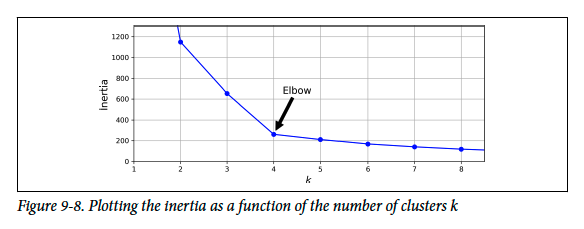
Elbow Method
The Elbow Method plots inertia as a function of .
Silhouette Score
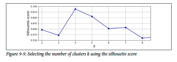
A more precise method is the Silhouette Score, which is the mean silhouette coefficient across all instances.
For an instance, the silhouette coefficient is:
where:
- = mean distance to the other instances in the same cluster, also called the mean intra-cluster distance
- = mean distance to the instances in the nearest neighboring cluster, excluding the instance's own cluster
The silhouette coefficient ranges from to .
- Close to → the instance is well inside its own cluster and far from other clusters
- Close to → the instance is near a cluster boundary
- Close to → the instance may have been assigned to the wrong cluster
from sklearn.metrics import silhouette_score
silhouette_score(X, kmeans.labels_)
To choose , compute the silhouette score for several possible values of and compare them.
Silhouette Diagram
A Silhouette Diagram provides more detail by displaying the silhouette coefficient of every instance, grouped by cluster.
Each cluster appears as a knife-shaped region:
- Height → number of instances in the cluster
- Width → silhouette coefficients of the instances
- Wider toward → better-separated instances
A vertical dashed line represents the mean silhouette score.
If many instances in a cluster fall to the left of the mean silhouette score, the cluster may be poorly defined because many of its instances are too close to another cluster.
In the example:
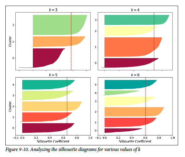
- and produce relatively poor clusters.
- and produce good clusters.
- Although has a slightly higher overall silhouette score, its cluster sizes are uneven.
- With , the clusters have more similar sizes, so choosing may still be preferable.
Note.
The best is not always determined by a single metric. Inertia, silhouette score, cluster balance, and the practical meaning of the clusters should all be considered.
Limits of K Means
K Means is fast and scalable, but has important limitations. It may need several runs to avoid poor local solutions, requires specifying the number of clusters , and performs poorly when clusters have different sizes, densities, or nonspherical shapes.
For elongated or ellipsoidal clusters, K Means may split natural clusters or merge parts of different clusters. A solution with lower Inertia is not necessarily the most meaningful clustering. Gaussian Mixture Models often work better for ellipsoidal clusters.
Warning.
Scale input features before using K Means. Since clustering depends on Euclidean distance, features on larger scales can dominate the distance calculation. Scaling helps, but K Means still generally prefers spherical clusters.
Using Clustering for Image Segmentation
Image Segmentation partitions an image into multiple segments.
- Color segmentation groups pixels with similar colors into the same segment.
- Semantic segmentation groups pixels belonging to the same object type. For example, all pedestrian pixels belong to the pedestrian segment.
- Instance segmentation separates individual objects, so each pedestrian would receive a different segment.
Modern semantic and instance segmentation generally use complex neural network architectures. This section instead uses K Means for simpler color segmentation.
Loading an Image
import PIL
image = np.asarray(PIL.Image.open(filepath))
image.shape
The image is a 3D array with shape (height, width, channels). Here there are 3 RGB channels. Each pixel is represented by red, green, and blue intensities stored as unsigned 8 bit integers from to .
Color Segmentation with K Means
X = image.reshape(-1, 3)
kmeans = KMeans(n_clusters=8, random_state=42).fit(X)
segmented_img = kmeans.cluster_centers_[kmeans.labels_]
segmented_img = segmented_img.reshape(image.shape)
image.reshape(-1, 3) converts the image into one row per pixel, with RGB as the 3 features.
K Means groups the pixel colors into n_clusters=8 color clusters. kmeans.labels_ gives the cluster assigned to each pixel.
kmeans.cluster_centers_[kmeans.labels_]
replaces every pixel with the RGB value of its cluster centroid, effectively reducing the image to 8 representative colors.
The result is then reshaped back to the original image dimensions.
Using fewer color clusters produces stronger color compression. However, small objects may disappear because K Means tends to favor clusters of similar sizes. In the ladybug example, when too few clusters are used, the small red ladybug is merged with surrounding colors.
Using Clustering for Semi Supervised Learning
Semi Supervised Learning is useful when there are many unlabeled instances but only a small number of labeled ones. The example uses Scikit Learn's digits dataset containing 1,797 grayscale images representing digits through .
from sklearn.datasets import load_digits

X_digits, y_digits = load_digits(return_X_y=True)

X_train, y_train = X_digits[:1400], y_digits[:1400]
X_test, y_test = X_digits[1400:], y_digits[1400:]
Baseline with Only 50 Labeled Instances
from sklearn.linear_model import LogisticRegression
n_labeled = 50
log_reg = LogisticRegression(max_iter=10_000)
log_reg.fit(X_train[:n_labeled], y_train[:n_labeled])
log_reg.score(X_test, y_test)
Training on only the first 50 labeled instances gives about accuracy.
Selecting Representative Instances
Instead of labeling 50 arbitrary instances, cluster the training set into 50 clusters and select the training image closest to each centroid.
k = 50
kmeans = KMeans(n_clusters=k, random_state=42)
X_digits_dist = kmeans.fit_transform(X_train)
representative_digit_idx = np.argmin(X_digits_dist, axis=0)
X_representative_digits = X_train[representative_digit_idx]
X_digits_dist contains the distance from every training image to every centroid.
np.argmin(X_digits_dist, axis=0) finds the training image with the smallest distance to each centroid, giving one representative image per cluster.
After manually labeling these representatives:
y_representative_digits = np.array([1, 3, 6, 0, 7, 9, 2, ..., 5, 1, 9, 9, 3, 7])
train Logistic Regression on them:
log_reg = LogisticRegression(max_iter=10_000)
log_reg.fit(X_representative_digits, y_representative_digits)
log_reg.score(X_test, y_test)
Accuracy improves from about to while still manually labeling only 50 images.
Important.
When manual labeling is expensive, labeling representative instances can be much more useful than labeling randomly selected instances.
Label Propagation
Label Propagation assigns the representative label of each cluster to all other instances in that cluster.
y_train_propagated = np.empty(len(X_train), dtype=np.int64)

for i in range(k):
    y_train_propagated[kmeans.labels_ == i] = y_representative_digits[i]
For cluster , every training instance satisfying kmeans.labels_ == i receives y_representative_digits[i].
Train again using all training instances with their propagated labels:
log_reg = LogisticRegression()
log_reg.fit(X_train, y_train_propagated)
log_reg.score(X_test, y_test)
Accuracy increases to about .
Removing the Least Representative Instances
Some points far from their centroid may be outliers or may not truly belong to the representative's class. The next step keeps only the closest of instances within each cluster.
percentile_closest = 99
X_cluster_dist = X_digits_dist[np.arange(len(X_train)), kmeans.labels_]

for i in range(k):
    in_cluster = (kmeans.labels_ == i)
    cluster_dist = X_cluster_dist[in_cluster]
    cutoff_distance = np.percentile(cluster_dist, percentile_closest)
    above_cutoff = (X_cluster_dist > cutoff_distance)

    X_cluster_dist[in_cluster & above_cutoff] = -1
X_cluster_dist stores each training instance's distance to the centroid of the cluster it belongs to.
For each cluster, distances above the 99th percentile are marked as -1.
partially_propagated = (
    X_cluster_dist != -1
)
X_train_partially_propagated = X_train[partially_propagated]
y_train_partially_propagated = y_train_propagated[partially_propagated]
The farthest of instances in every cluster are removed. Train again:
log_reg = LogisticRegression(max_iter=10_000)
log_reg.fit(X_train_partially_propagated, y_train_partially_propagated)
log_reg.score(X_test, y_test)
Accuracy reaches about , slightly better than training on the fully labeled dataset in this example.
The quality of the propagated labels can be checked against the true labels:
(
    y_train_partially_propagated
    == y_train[partially_propagated]
).mean()
About of the retained propagated labels are correct.
Scikit Learn also provides LabelSpreading and LabelPropagation, which automatically propagate labels from labeled to similar unlabeled instances.
SelfTrainingClassifier takes a base classifier, predicts labels for unlabeled instances, adds the predictions it is most confident about to the training set, then repeats this process.
Active Learning
Active Learning involves interaction between the learning algorithm and a human expert. The algorithm chooses which instances would be most useful to label.
A common strategy is uncertainty sampling:
- Train the model on the labeled instances available so far and predict the unlabeled instances.
- Ask an expert to label the instances for which the model is most uncertain, such as those with the lowest predicted probability.
- Repeat until the improvement is no longer worth the labeling effort.
Other strategies may select instances expected to cause the largest model change, reduce validation error the most, or expose disagreement between different models.
DBSCAN
DBSCAN (density based spatial clustering of applications with noise) defines clusters as continuous regions of high density.
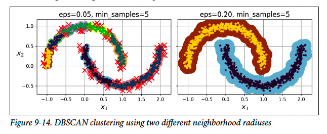
For each instance, DBSCAN counts how many instances lie within distance (eps). This region is the instance's neighborhood.
An instance is a core instance if its neighborhood contains at least min_samples instances, including itself. All instances in the neighborhood of a core instance belong to the same cluster. Neighboring core instances can therefore form long connected clusters.
An instance that is not a core instance and has no core instance in its neighborhood is considered an anomaly or noise.
DBSCAN works well when clusters are separated by low density regions.
from sklearn.cluster import DBSCAN
from sklearn.datasets import make_moons

X, y = make_moons(n_samples=1000, noise=0.05)
dbscan = DBSCAN(eps=0.05, min_samples=5)
dbscan.fit(X)
eps=0.05 defines the neighborhood radius, while min_samples=5 requires at least 5 nearby instances for an instance to become a core instance.
dbscan.labels_
labels_ contains the cluster assigned to every instance. A label of -1 indicates an anomaly.
dbscan.core_sample_indices_
core_sample_indices_ contains the indices in X of the core instances.
dbscan.components_
components_ contains the actual feature values of the core instances, approximately equivalent to X[dbscan.core_sample_indices_].
Increasing eps widens each instance's neighborhood. In the moons example, eps=0.05 creates several clusters and anomalies, while eps=0.20 connects the points within each moon and produces two clean clusters.
Note.
min_samplescontrols the minimum local density, not the number of clusters. DBSCAN automatically determines the number of clusters from connected dense regions.
Predicting New Instances
DBSCAN has fit_predict() but no predict() method. A separate classifier can be trained using the discovered clusters.
from sklearn.neighbors import KNeighborsClassifier
knn = KNeighborsClassifier(n_neighbors=50)
knn.fit(dbscan.components_, dbscan.labels_[dbscan.core_sample_indices_])
This trains K Nearest Neighbors using only the DBSCAN core instances and their discovered cluster labels.
X_new = np.array([[-0.5, 0], [0, 0.5], [1, -0.1], [2, 1]])
knn.predict(X_new)
knn.predict_proba(X_new)
The classifier can assign new instances to the discovered clusters and estimate cluster probabilities. However, because the KNN classifier was trained without an anomaly class, it always assigns a cluster even to distant instances. A maximum distance threshold can be added manually.
y_dist, y_pred_idx = knn.kneighbors(X_new, n_neighbors=1)
y_pred = dbscan.labels_[dbscan.core_sample_indices_][y_pred_idx]
y_pred[y_dist > 0.2] = -1
y_pred.ravel()
Instances farther than 0.2 from their nearest core instance are marked as anomalies with -1.
DBSCAN Summary
DBSCAN can identify any number of clusters with arbitrary shapes and is robust to outliers. Its main hyperparameters are eps and min_samples.
Warning.
DBSCAN may struggle when cluster densities vary significantly or when clusters are not separated by sufficiently low density regions. Its computational complexity is roughly , so it does not scale well to very large datasets.
HDBSCAN is a hierarchical extension that generally handles clusters with varying densities better than standard DBSCAN.
Other Clustering Algorithms
Agglomerative Clustering
Agglomerative Clustering builds a hierarchy of clusters from the bottom up. It starts with individual instances and repeatedly merges the nearest pair of clusters.
The result can be represented as a tree whose leaves are individual instances. It can capture clusters of various shapes and supports arbitrary pairwise distance measures.
A connectivity matrix can restrict which instances are allowed to be considered neighbors. This can improve scalability, but without such a matrix the algorithm does not scale well to large datasets.
BIRCH
BIRCH (balanced iterative reducing and clustering using hierarchies) is designed for very large datasets.
It builds a compact tree structure containing enough information to assign new instances to clusters without storing every training instance. This enables limited memory usage and can be faster than batch K Means when the number of features is relatively small, roughly fewer than 20.
Mean Shift
Mean Shift begins by placing a circle around every instance. Each circle is repeatedly shifted toward the mean of the instances it contains.
This moves the circles toward regions of higher density until they converge near local density maxima. Instances whose circles converge to the same location are assigned to the same cluster.
Mean Shift can discover any number of arbitrarily shaped clusters and relies on only one main hyperparameter: the circle radius, called the bandwidth.
Warning.
Mean Shift may split clusters when their internal densities vary. Its computational complexity is , making it unsuitable for large datasets.
Affinity Propagation
Affinity Propagation repeatedly exchanges messages between instances until each instance chooses another instance, or itself, to represent it.
The selected representatives are called exemplars. Each exemplar and the instances choosing it form a cluster.
Unlike K Means, the number of clusters does not need to be specified beforehand; it is determined during training. Affinity Propagation also handles clusters of different sizes reasonably well.
Warning.
Computational complexity is , so Affinity Propagation is not suitable for large datasets.
Spectral Clustering
Spectral Clustering starts with a similarity matrix between instances and creates a lower dimensional embedding from it. Another clustering algorithm, such as K Means, is then applied in this transformed space.
It can capture complex cluster structures and can also be used for graph partitioning, such as identifying communities in a social network.
Warning.
Spectral Clustering does not scale well to large numbers of instances and performs poorly when clusters have very different sizes.
Gaussian Mixtures
A Gaussian mixture model (GMM) is a probabilistic model that assumes the data was generated from a mixture of Gaussian distributions with unknown parameters. Each Gaussian component generally corresponds to an ellipsoidal cluster and may have its own location, size, density, shape, and orientation.
For each instance :
- A cluster is selected with probability , where is the cluster's weight. The hidden cluster assignment is denoted .
- If , the instance is sampled from that cluster's Gaussian distribution: , where is the mean and is the covariance matrix.
Given only the observed dataset , the goal is to estimate the cluster weights , means , and covariance matrices .
from sklearn.mixture import GaussianMixture

gm = GaussianMixture(n_components=3, n_init=10)
gm.fit(X)
The estimated parameters are available through learned attributes:
gm.weights_      # relative weight of each Gaussian component
gm.means_        # mean vector of each component
gm.covariances_  # covariance matrix of each component
Expectation Maximization
GaussianMixture uses the Expectation Maximization (EM) algorithm. It is similar to K Means but uses soft assignments rather than assigning each instance to exactly one cluster.
EM initializes the cluster parameters, then alternates between two steps until convergence:
- Expectation step: estimate the probability that each instance belongs to each cluster using the current parameters.
- Maximization step: update each cluster's weight, mean, and covariance using all instances, weighted by their estimated probabilities of belonging to that cluster.
These estimated cluster membership probabilities are called responsibilities. A cluster's parameters are influenced most strongly by the instances for which it has high responsibility.
Warning.
Like K Means, EM may converge to a poor local solution.
n_initcontrols how many initializations are tried, keeping the best solution. The source recommends settingn_initto a sufficiently large value rather than relying on the default.
gm.converged_  # True if EM converged
gm.n_iter_     # number of EM iterations performed
Hard and Soft Clustering
Once the model is fitted, it can perform either hard or soft clustering.
gm.predict(X)                 # hard clustering: most likely component
gm.predict_proba(X).round(3)  # soft clustering: probability for each component
predict() assigns each instance to its most likely Gaussian component, while predict_proba() returns the estimated responsibility of every cluster for each instance.
Generating New Instances
A GMM is a Generative Model, so it can generate new samples from the learned mixture.
X_new, y_new = gm.sample(6)
X_new contains generated instances, while y_new contains the Gaussian component used to generate each one.
Probability Density
A fitted GMM can estimate the density of the learned distribution at any location.
gm.score_samples(X).round(2)
score_samples() returns the log probability density for each instance. Higher values indicate locations with greater estimated density.
If is returned by score_samples(), then gives the actual PDF value.
Note.
A probability density is not itself a probability and may exceed . To obtain the probability of an instance falling inside a region, integrate the PDF over that region.
The density contours of a trained GMM reflect the learned Gaussian components, while decision boundaries indicate which component has the highest responsibility in each region.
Covariance Constraints
When there are many features, clusters, or instances, estimating a full covariance matrix for every Gaussian can become difficult. covariance_type can constrain the possible cluster shapes and reduce the number of learned parameters.
covariance_type | Constraint |
|---|---|
"spherical" | Every cluster is spherical, but clusters may have different variances and therefore different diameters |
"diag" | Clusters may be ellipsoidal with different sizes, but their axes must remain parallel to the coordinate axes; covariance matrices are diagonal |
"tied" | All clusters share the same covariance matrix, so they have the same ellipsoidal shape, size, and orientation |
"full" | Default; every cluster has its own unrestricted covariance matrix and may have its own shape, size, and orientation |
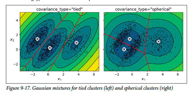 | |
"full" is the most flexible but also learns the most parameters. |
Computational complexity depends on the number of instances , features , clusters , and covariance constraints. With "spherical" or "diag", training is roughly . With "tied" or "full", it is roughly , so these settings do not scale well to very high dimensional data.
Using Gaussian Mixtures for Anomaly Detection
A GMM can perform Anomaly Detection by treating instances in low density regions as anomalies.
Choose a density threshold according to the expected anomaly rate. For example:
densities = gm.score_samples(X)
density_threshold = np.percentile(densities, 2)
anomalies = X[densities < density_threshold]
np.percentile(densities, 2) finds the 2nd percentile of density scores, so approximately the lowest density of instances are flagged as anomalies.
The threshold controls the usual precision and recall tradeoff:
- Too many false positives → lower the threshold.
- Too many false negatives → increase the threshold.
Novelty Detection differs from anomaly detection because novelty detection assumes the training data is clean and contains no outliers, while anomaly detection does not make this assumption.
Warning.
A GMM tries to fit all training data, including outliers. Too many outliers may distort its estimate of normality. One approach is to fit the model, remove the most extreme outliers, then fit it again on the cleaned data. Robust covariance estimation such as
EllipticEnvelopeis another option.
Selecting the Number of Clusters
Like K Means, GaussianMixture requires choosing the number of components in advance.
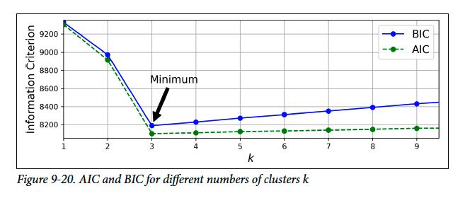
Inertia and Silhouette Score are less appropriate for GMMs because they are unreliable when clusters are nonspherical or have different sizes. Instead, choose the model that minimizes an information criterion such as BIC or AIC.
where is the number of instances, is the number of parameters learned by the model, and is the model's maximized likelihood.
Both BIC and AIC:
- Reward models that fit the data well through a larger likelihood.
- Penalize models with more parameters.
- Prefer the model with the lowest score.
BIC generally penalizes complexity more strongly than AIC. When they disagree, BIC therefore tends to select a simpler model with fewer parameters, while AIC may select a more complex model that fits the observed data better.
Likelihood Function
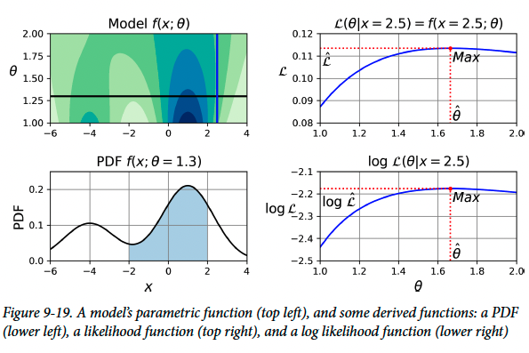
Consider a statistical model , where is the observed or possible data and represents the model parameters.
Definition (Probability density function (PDF)).
For a continuous random variable with parameter fixed, the PDF describes the relative density of possible outcomes . Probabilities are obtained by integration: , and .
The PDF is therefore a function of while is fixed.
In the example, the model is a 1D mixture of two Gaussian distributions centered at and , while the parameter controls their standard deviations. Fixing gives the PDF , which describes the density of possible values of .
Definition (Likelihood Function).
After observing data , the likelihood function treats as fixed and the model parameter as variable: . It measures how plausible different parameter values are given the observed data.
For example, after observing , the likelihood is . Varying shows which value makes the observation most plausible.
| Concept | Fixed | Variable | Main question |
|---|---|---|---|
| Given the model parameters, which outcomes are plausible? | |||
| Likelihood | Given the observed data, which parameter values are plausible? |
Important.
A likelihood function is not a probability distribution over . A PDF integrates to over all possible , but is not required to equal .
Maximum Likelihood Estimation
Definition (Maximum likelihood estimation (MLE)).
Maximum likelihood estimation (MLE) chooses the parameter value that maximizes the likelihood of the observed data: .
denotes the maximum likelihood estimate of .
In the example with the single observation , the likelihood is maximized at approximately .
For independent observations , the joint likelihood is the product of the individual likelihoods: .
Log Likelihood
Definition (Log Likelihood).
Log Likelihood is the logarithm of the likelihood: .
Because is strictly increasing, maximizing the likelihood and maximizing the log likelihood give the same .
For independent observations, logarithms convert the product of likelihoods into a sum: , using .
This is usually easier and more numerically convenient to optimize than multiplying many individual likelihood values.
Maximum A Posteriori Estimation
Definition (Maximum a posteriori estimation (MAP)).
Maximum a posteriori estimation (MAP) incorporates a prior distribution and chooses by maximizing .
MLE uses only the observed data, while MAP also incorporates prior beliefs about plausible parameter values. Because the prior constrains the parameters, MAP can be viewed as a regularized form of MLE.
Maximized Likelihood
After estimating , the maximized likelihood is .
measures how well the fitted model explains the observed data and is later used when computing AIC and BIC.
Selecting the Number of Clusters
For a fitted Gaussian Mixture Model, Scikit Learn provides bic() and aic():
gm.bic(X)  # 8189.747000497186
gm.aic(X)  # 8102.521720382148
Bayesian Gaussian Mixture Models
Instead of manually searching for the optimal number of clusters, BayesianGaussianMixture can automatically reduce the importance of unnecessary components by assigning them weights close to .
Set n_components to a value believed to be larger than the true number of clusters. The model can effectively eliminate unnecessary components.
from sklearn.mixture import BayesianGaussianMixture

bgm = BayesianGaussianMixture(n_components=10, n_init=10, random_state=42)
bgm.fit(X)
bgm.weights_.round(2)  # array([0.4, 0.21, 0.4, 0., 0., 0., 0., 0., 0., 0.])
Although 10 components were allowed, only about 3 received meaningful weights, so the model effectively discovered that only 3 clusters were needed.
Warning.
Gaussian mixture models work well for ellipsoidal clusters but may perform poorly on clusters with very different or arbitrary shapes. On the moons dataset, the model tries to approximate the curved moons using several ellipsoidal Gaussian components instead of identifying the two natural moon shaped clusters.
Other Algorithms for Anomaly and Novelty Detection
Fast MCD
Fast MCD or minimum covariance determinant is implemented by EllipticEnvelope and is useful for Outlier Detection, particularly for cleaning datasets.
It assumes that normal instances come from a single Gaussian distribution and that some observations are outliers generated differently.
The algorithm estimates the Gaussian parameters while trying to ignore likely outliers, producing a more robust estimate of the elliptical region containing normal instances.
Isolation Forest
Isolation Forest is efficient for outlier detection, especially in high dimensional datasets.
It builds random decision trees. At each node, it randomly selects a feature and then randomly selects a threshold between that feature's minimum and maximum values.
The data is progressively split until instances become isolated.
Note.
Anomalies tend to be easier to isolate than normal instances, so across the forest they usually require fewer splits to become isolated.
Local Outlier Factor
Local Outlier Factor (LOF) detects anomalies by comparing the local density around an instance with the density around its neighbors.
An instance is considered suspicious when its neighborhood is significantly less dense than the neighborhoods of its nearest neighbors.
One Class SVM
One Class SVM is especially suited for Novelty Detection.
A kernelized SVM implicitly maps the training instances into a higher dimensional feature space. Since only one normal class is available, One Class SVM attempts to separate these instances from the origin.
In the original feature space, this corresponds to finding a small region that contains the normal training instances. A new instance outside this region is considered novel or anomalous.
It works particularly well with high dimensional datasets but, like other SVM methods, does not scale well to very large datasets.
PCA and Reconstruction Error
PCA and other dimensionality reduction methods that support inverse_transform() can also be used for anomaly detection.
A normal instance should be reconstructed reasonably well after dimensionality reduction and inverse transformation. An anomalous instance generally has a larger reconstruction error.
Note.
Large reconstruction error can therefore serve as an anomaly score.